In current market, it is always required to move with time. In fact, calculate or assess the future is in demand in all the industries, be it retail or ecommerce or software industry. The concept of Time Series forecasting plays a very important role in calculating future values.
There are number of ways to predict future value, as an example take previous three value’s average and add this in the last value, it will give you future value. Defiantly it is a good method but does not consider all the features of the data set as in trend, seasonality, white noise etc.
Oh, I used so many terms. Let me explain what the meaning of these terms are.
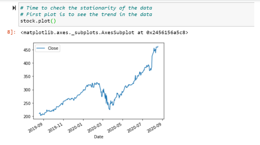
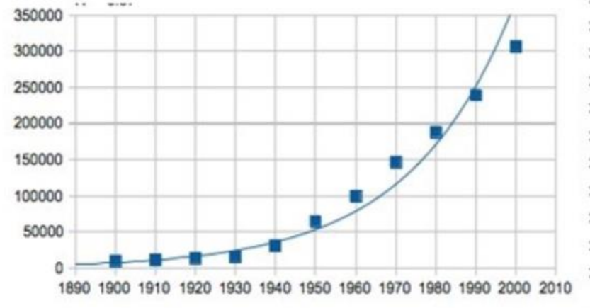
1) Trend : We see the graph of our data, we see it moving upward or downward or in pattern. We call it trend. Suppose, we started a business of producing toys. In the first year we were not able sell good amount of toys but next year we sold more than last year. Again next year number if more than last year. So, we see an upward increasing trend in the sales number.
2) Seasonality: I will start with a question. When do we buy swimming dress? In winter or in
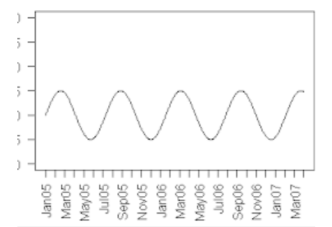
summer? We buy it in winter right. We buy car or costly things during festival season, because we hope to get some discount during that time period. This is called seasonality in data. The peak reaches in a certain time period of the year. In the following diagram, we see some seasonality which is occurring after every certain time period. We must have studied something called periodic occurrence of an event. Seasonality is nothing but periodic occurrence of an event. That event may be sales value, demand of product, share price, Medicine requirement etc.
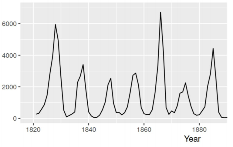
3) Cyclic data: This is another kind of data which we will encounter while doing time series
forecasting.
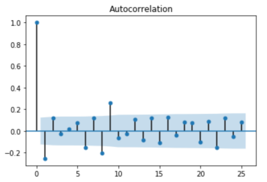
4) White Noise: Time series data in which there is no correlation is called white noise. For white noise, each auto-correlation should be close to zero. One thing to note here, as there will be some random variation so auto-correlation will not be exactly zero.
A very important concept called stationarity of the data, without which we can not perform time series data analysis and forecasting. Let us understand what is stationarity of the data:
In the most intuitive sense, stationarity means that the statistical properties of a process generating a time series do not change over time. Stationary process is easier to analyze. To check the stationarity of the data, we perform Augmented Dickey Fuller test. This test is based on the null hypothesis which says the data is non-stationary. Hence, if the p-value comes less than significance level (0.05), then we reject the null hypothesis and conclude the data is stationary. But, if the p-value is greater than 0.05, the we can not reject the null hypothesis and conclude that the data is non-stationary. Now to make the data
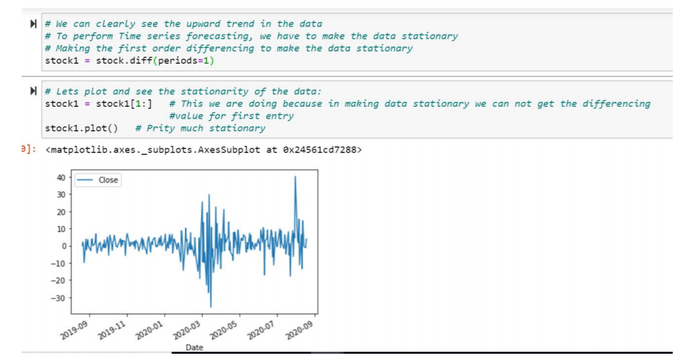
stationary, we perform method of differencing. We use the concept of differencing to make data stationary and call it as data is Integrated of Order d ( d = 1,2,3…).
Let’s understand the term “Data is Integrated of Order 1”. Suppose we have share price of any share till today. To make data stationary, we subtract todays share price from yesterday’s share price, yesterday’s share price is subtracted from day before yesterday’s share price and so on. So, if we are taking one time period lag, then it is called Data is integrated of Order 1.
The widely used Time series model is called ARIMA model. ARIMA stand for Autoregressive Integrated Moving Average. As the name suggest, ARIMA model has three different components. 1)Autoregressive 2) Integrated and 3) Moving Average. These three components are characterized by three terms: p, d, q. Let us understand these three components separately. The terms integrated is explained above and it is indicated by d.
Autoregressive is a model, in which we predict the future value based on the past value. Let’s consider the share price that we want to predict for tomorrow. So, we can predict the share price for tomorrow, based on the share price for today. We do not need any other variable. So, if we predict the value of a variable based the past value of same variable, it is called Autoregression.
Yt=b0+aY(t-1)+cY(t-2) In this equation we are predicting y value at time t based on the time (t-1)and(t-2). So, we are taking two previous terms to predict future y. So, number of previous terms taken to predict future value is called the order and in case of Autoregressive it is indicated by p. in our example, p = 2.
Another concept is Moving average. In this we build the same equation but based on the error.
Yt=b+εt +θ0ε(t-1) +..
Here εt is the error calculated at time t. i.e. the difference between predicted value and actual value of Y at time t. similarly ε(t-1) is the error calculated at time (t-1). So, the number of error terms taken in the moving average equation is called the order of moving average and is indicated by q. Here q = 2.
If we will combine these two model, we will ger Autoregressive moving average model (ARMA): Yt=(b0+b+εt)+(aY(t-1)+θ0ε(t-1) )+…..
This model is considered very efficient model in building Time Series analysis. But our data should be Stationary. So, if our data is stationary then it is good or else, we apply the method of differencing to make the data stationary and then the model is called ARIMA.
In all, three terms p,d,q indicates the orders of AR, Integrated (to make the data stationary) and Moving average. It is important to note here that, to make the data stationary, we should use differencing but, we should be careful that we should not use over-differencing. Because, an over differenced series may still be stationary. Which in turn will affect the model parameters.
Note: Another method to make the data stationary is the transformation. Generally, log transformation is used to make the data stationary. But, the most preferred way is differencing.
Now, hoe to find the order of the AR term (p)?
We can find out the required number of AR terms by inspecting the partial Autocorrelation (PACF) plot. Any autocorrelation in a stationarized series can be rectified by adding enough AR terms. So, we initially take the order of AR term to be equal to as many lags that crosses the significance limit in the PACF plot.
How to find the order of the MA term (q)?
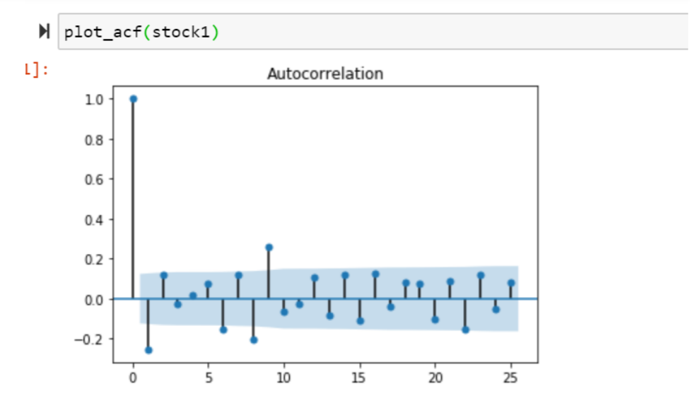
We can see the ACF plot for the number of MA terms. An MA term is technically, the error of the lagged forecast. The ACF tell how many MA terms are required to remove any autocorrelation in the stationarized series.
Evaluation of the model:
Once the model is built, we can evaluate the model with different matrices. Like Mean Absolute percentage error (MAPE), Mean Error (ME), Mean absolute error (MAE), Mean Squared error (MSE), root mean squared error (RMSE). But an alternative is to use what is called information criteria (IC). There are many criteria and the most common are Akaike’s Information Criteria (AIC). The fact that more complex model is typically able to fit better to past data, to the extent it may overfit. If it overfits then it will not produce good forecasts from unseen future data. IC is trying to balance how good a model fits and its complexity. In general,
IC = goodness of fit + Penalty for model complexity
Model complexity is typically the number of model parameters scaled by some factor to make it comparable to the goodness of fit metric, which itself is based on the idea of the likelihood function.
AIC = 2k – 2ln(L)
Here, k is the number of model parameters, L is the likelihood function. The likelihood function is a function of MSE. Which modifies the AIC equation as:
AIC = 2k + n ln(MSE) ; where is n is the sample size.
As, we know a model that fits well will have small MSE. If to do that, it needs a lot of model parameters (complexity), then the term 2k will be large, thus making AIC large. Hence, we will always want a model with low AIC value, which will take care of the model complexity and the MSE also. Hence, it will lead to less chance of overfitting. So, in case of AIC there is no need of validation required. Hence, we will have more data to train the model.
Let us do some coding:
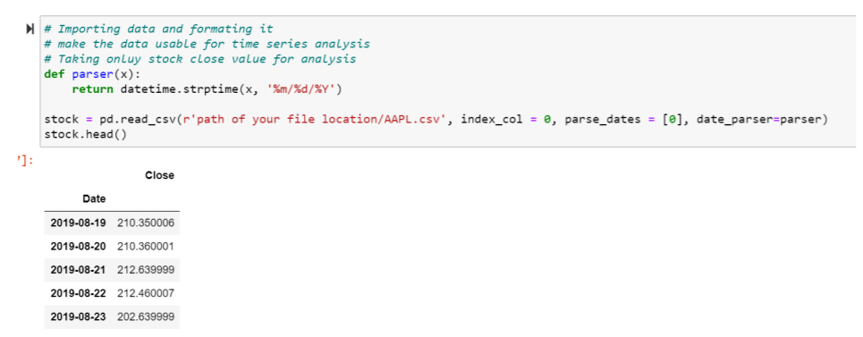
Step 1 : Data fetching : https://finance.yahoo.com/quote/AAPL/history?p=AAPL
This is the data source where I am taking historical data of Apple Inc. This is one year data of the share price of Apple company.
I have downloaded the data into my local system. If you want to, then you can directly read the data from website.

