Just like Mathematics and Physics, Statistics and Machine learning go hand in
hand. They are both used to get insights from the Data. In this blog, I’ll discuss
some crucial concept of statistics which are widely used in ML and give a brief
introduction to each of the topics.
Table of Content
- Probability Basics.
- Sample and Sampling Distribution
- Central Limit Theorem
- Hypothesis Testing and P-values
- Covariance and Correlation
- T-tests
- Regression and ANOVA
1. Probability Basics
If E represents an event, P(E) represents the Probability of occurrence of the event.
P(E) = number of favourable outcomes / total outcome in the sample space.
• Random Variable: If the outcome of the event (like tossing a coin or rolling a die) is random, then the variable that represents the outcome of these events is called a random variable.
• Joint probability: The probability of occurrence of two independent events A and B is given by P(A and B) or P(A ∩ B).
P(A ∩ B) = P(A). P(B)
• Conditional Probability: The probability of occurrence of two dependent events A and B is given by P(A|B).
P(A|B) = P(A ∩ B)/ P(B)
• Bayes’ Theorem: This theorem helps us calculate the likelihood of a occurrence an event under given condition.
P(A|B) = (P(B|A) . P(A)) / P(B)
Where,
P(A|B): Probability of A given B is true
P(B|A): Probability of B given A is true
P(A),P(B): independent probabilities of A and B respectively
• Mean, Median and Mode : Mean is the arithmetic mean of the data whereas Median is the middle data value given that data is sorted. The data value that has the most frequency is the mode
• Variance: measures how far each number in the set is from the mean. It is the squared difference from mean
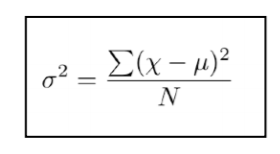
Where, x is a data point, µ is the mean of all data and N is the total number of data.
• Standard Deviation: this defines the width of the normal distribution’s curve. It is square root of variance.
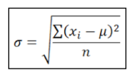
Where symbols have their usual meaning (as stated above).
• Z-score: The Z-score for a particular data value represents how many standard deviations the data value lies above or below the mean.
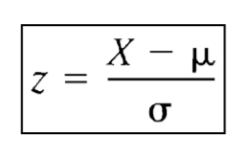
Where X is the data point, µ is mean and sigma is the standard deviation.
• R-squared: r-squared shows how well the data fit the regression model.
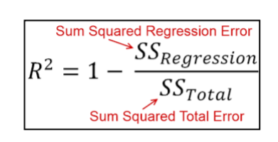
**regression model: This model is used to investigate relationship between one or more variables and estimate one variable given the other.
2. Sample And Sampling Distribution
• Population: The entire pool of a data set is known as Population. For example, group of people, objects, events, etc.
• Sample : A small set of group collected from statistical population is known as sample. Since, we don’t have time and money to calculate population mean to entire data set, we take a sample and estimate population mean.
• Population and Sample Parameters: Standard deviation and mean are the parameters for population and sample .
Population mean (µ) = ( Σ Xi ) / N
Population SD (σ) = sqrt[ Σ ( Xi – µ )2 / N ]
Where, Σ Xi is sum of all individual data present in the population and N is the total number of individuals or data in the population.
Sample mean (x̄) = ( Σ xi ) / n
Sample SD (s) = sqrt [ Σ ( xi – x_bar )2 / ( n – 1 ) ]**
Where, Σ xi is sum of all individual data present in the sample and n is the total number of individuals or data in the sample.
**the (n-1) compensates for the fact that we are calculating difference from the sample and not population.
• Sampling Distribution: A Sampling Distribution is a probability distribution (curve) of a statistic obtained through a large number of samples drawn from a specific population.
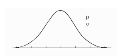
The shape of the distribution does not reveal anything about the shape of the population. It is just used to estimate the population statistics by using Central Limit Theorem which we will discuss next.
3. Central Limit Theorem
In simple language, this theorem states that, even if the means are calculated using data from different distributions, like uniform or exponential, the means themselves are not uniformly distributed. Instead, they are normally distributed. This will be clear with some illustrations!
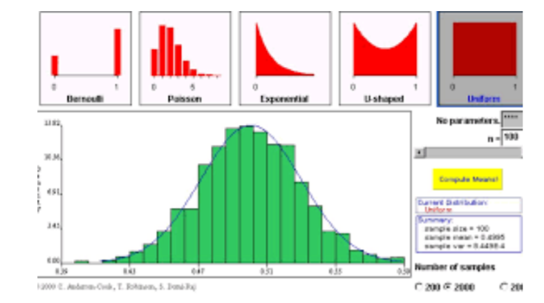
In the above figure, the red graphs represents different distributions of data. The green graph is the mean of each of those distributions suggesting that mean is always normally distributed irrespective of the data distribution.
4. Hypothesis Testing And P-value
• Hypothesis : A hypothesis is an educated guess about something in the world around you. It should be testable, either by experiment or observation. For example, a drug A might be effective again the virus.
• Hypothesis Testing: Hypothesis testing in statistics is a way to test the results of a survey or experiment to see if we have meaningful results. Technically, It lets a sample statistic to be checked against a population statistic or statistic of another sample to study any intervention etc.
• Null Hypothesis: It is the hypothesis where there is no difference between sample statistics and population statistics i.e. they are same. For example, Drug A and Drug B have same effect against the virus. We can either reject or fail to reject a Null hypothesis.
• Alternate Hypothesis: It states opposite of Null hypothesis. From above Null Hypothesis, the alternative would be: Drug A and Drug B have different effect against the virus.
• P-values: it is the probability of obtaining results at least as extreme as the observed results of a statistical hypothesis test, assuming that the null hypothesis is correct. A smaller p-value means that there is stronger evidence in favour of the alternative hypothesis.
P-values helps us decide to reject a Null hypothesis or not. If p-val is <0.05 then we reject it.
• Calculating P-value: A p-value is of two types: one-sided and two sided and
is sum of three parts:
- The probability random chance would result in observation.
- The probability of observing something else that is equally
rare. - The probability rarer or more extreme.
For example, the p-value for getting 2 heads on flipping 2 coins is:
P-value = 0.25 + 0.25 + 0 = 0.5
Where, first 0.25 is probability of getting 2 heads, second 0.25 is probability of getting something equally rare, in this case it is getting 2 tails.
0 is the probability of observing something more rarer than getting 2 head and 2 tails which in this case is none.
5. Covariance and Correlation
• Covariance: covariance is a measure of the relationship between two random variables i.e. the joint variability of two random variables.

where,
Xi = data value of x
Yi = data value of
x̅ = mean of x
y̅ = mean of y
n = number of data values
• Trends: There are three ways in which two random variables are related to each other:
- Positive trend: if the slope between the random variables is positive then it shows positive trend.

2. Negative trend: if the slope between the random variables is negative, then it shows negative trend.
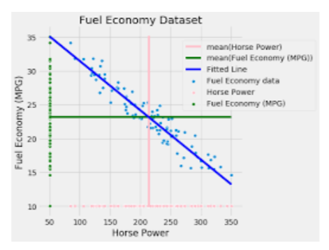
3. No trends: the random variables are not related to each other i.e. they do not increase or decrease while other changes. The graph is a straight line parallel to any of the axis.
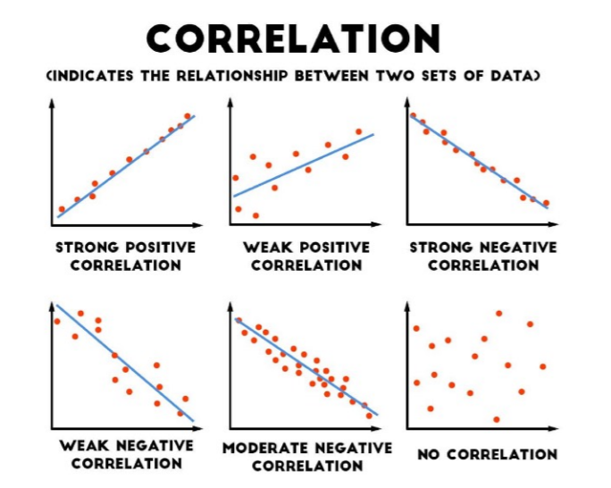
• Correlation: Correlation provides direction as well as strength of the relationship between two random variables.
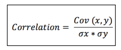
where,
Cov(x,y) = covariance of x and y
σ(x) = standard deviation of x
σ(y) = standard deviation of y
• Types of Correlation: Since, correlation quantifies the strength, it can classified into 3 categories:
- Weak Relationship : small correlation value
- Moderate Relationship : moderate correlation value
- Strong Relationship : Large correlation value
6. T-tests
• T-tests are very much similar to the z-scores, the only difference being that instead of the Population Standard Deviation, we now use the Sample Standard Deviation. The rest is same as before, calculating probabilities on basis of t-values.
• t-values are dependent on Degree of Freedom of a sample.
• Degree of freedom: It is the number of variables that have the choice of having more than one arbitrary value. For example, in a sample of size 10 with mean 10, 9 values can be arbitrary but the 10th value is forced by the sample mean.
Types of t-tests
1.1-sample t-test: This test determine whether the mean of a group differs from the specified value and calculate a range of values that are likely to include the population mean.
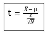
Where,
x̄ = sample mean,
µ = population mean
S = sample standard deviation
N = sample size
2. Paired t-test: Paired t-test is performed to check whether there is a difference in mean after a treatment on a sample in comparison to before. It checks whether the Null hypothesis: The difference between the means is Zero, can be rejected or not.
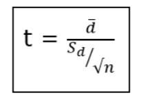
Where,
d̄ = mean of the case wise difference between before and after,
Sd = standard deviation of the difference
n = sample size
3. 2-sample t-test: This test determine whether the means of two independent groups differ and calculate a range of values that is likely to include the difference between the population means.
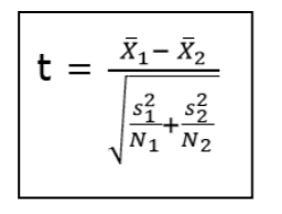
Where,
X̄1 = mean of first group
S1 = sample standard deviation of first group
N1 = represent sample size of first group
7. Regression and ANOVA
In Regression, we generally, calculate the weights for features present in the model to better predict the output variable. But finding the right set of feature weights or features for that matter is not always possible.
It is highly likely that that the existing features in the model are not fit for explaining the trend in dependent variable or the feature weights calculated fail at explaining the trend in dependent variable. What is important is knowing the degree to which our model is successful in explaining the trend (variance) in dependent variable.
With the help of ANOVA techniques, we can analyse a model performance very much like we analyse samples for being statistically different or not.
But with regression things are not easy. We do not have mean of any kind to compare or sample as such but we can find good alternatives in our regression model which can substitute for mean and sample.
Sample in case of regression is a regression model itself with pre-defined features and feature weights whereas mean is replaced by variance(of both dependent and independent variables).
Through our ANOVA test we would like to know the amount of variance explained by the Independent variables in Dependent Variable VS the amount of variance that was left unexplained.
It is intuitive to see that larger the unexplained variance(trend) of the dependent variable smaller will be the ratio and less effective is our regression model. On the other hand, if we have a large explained variance then it is easy to see that our regression model was successful in explaining the variance in the dependent variable and more effective is our model. The ratio of Explained Variance and Unexplained Variance is called F-Ratio.
Different F-Ratios:
• Regression (Explained) Sum of Squares : It is defined as the amount of variation explained by the Regression model in the dependent variable.

• Residual Sum of Squares : It is defined as the amount of variation independent variable which is not explained by the Regression model.

• Total Sum of Squares (TSS) : It is defined as the ratio of the amount of variance explained by the regression model to the total variation in the data. It represents the strength of correlation between two variables.
TSS = RSS + ESS
• Correlation Coefficient: This is another useful statistic which is used to determine the correlation between two variables. It is simply the square root of coefficient of Determination and ranges from -1 to 1 where 0 represents no correlation and 1 represents positive strong correlation while -1 represents negative strong correlation.
Conclusion
This blog has come to an end. Over here I have discussed some basics of Statistics ,covering almost all the topics along with their introduction and formulas.
References
• towardscience.com
• analyticalvidhya.com
• Stat quest (YouTube)
• Khan Academy
You can follow me on Linkedin: https://www.linkedin.com/in/muskaan-maurya-727567192/
