
1. Sentiment Analysis
Let us get this started with the definition of sentiment analysis itself. What is sentiment analysis?
“Sentiment analysis (or opinion mining) is a natural language processing technique used to determine whether data is positive, negative or neutral.“
As stated, the main goal of this blog is to explore various methods for sentiment analysis on text data.
2. Why is sentiment analysis important?
Consider a scenario, where you want to review a product of your company based on customer reviews. These reviews from the customer can be obtained from different sources like emails, surveys, social media conversations, etc. and most of them will be unstructured. To analyze this large volume of data and check the number of positive responses and negative responses will be very time-consuming. Now image a case where a machine automatically takes all these reviews and groups them into positive and negative reviews. Great isn’t it? That is exactly what we are trying to achieve through this study.
3. Prerequisites
- Familiarization with the need of text featurization and some featurization techniques
- Familiarization with machine learning classification models like Logistic regression, naive bayes, xgboost, etc.
4. Dataset Analysis and Preprocessing
This is the section that requires a lot of analysis and exploration in the entire machine learning pipeline. In this section, we will discuss the dataset, the columns in the dataset, univariate and multivariate analysis of each feature, some basic data cleaning, and feature engineering.
4.1 Dataset
The dataset considered in this case study is the Amazon product reviews dataset. As the name suggests, this dataset contains the customer reviews of various products on Amazon.
4.2 Column Analysis
The data set contains 21 columns. The description of features are described below
- Product id- Unique id of the product
- Name of the product
- asins: amazon standard identification number
- brand: Amazon sub-brands
- categories which the product belongs to
- keys
- manufacturer of the product
- reviews.date
- reviews.date added- The data which the review is added
- reviews.dateSeen
- reviews.didPurchase
- reviews.doRecommend- if the customer recommends this product or not
- reviews.id- id of each review
- review.numHelpful- Number of users who find the review helpful
- reviews.rating- Rating of the review
- reviews.source URLs
- reviews.text- The reviews
- reviews.title – the title of the review
- reviews.userCity- The city of the user
- reviews.user province
- reviews.username’ – User name
Given these features, we aim to predict the category or polarity of each of the reviews. One important analysis which is to be done is finding the number of null or “Nan” entries for each of these columns. A feature with too many null values will not be useful for the prediction in most scenarios. Here also, the features with too many missing values are discarded in further analysis.
The output which we need to predict is the polarity of a given review – positive or negative. Since we are not given the polarity directly, we will convert the column called rating(having values from 1 to 5) and convert it into another feature which is polarity.
4.3 Univariate analysis
Univariate analysis is done for each of the features using Box plots. This was used to determine how well each of these features contributes to predicting the reviews. Using a box plot, potential outliers can also be determined. If a feature can distinguish the polarities of reviews, then that feature can be useful for the prediction. This can be explained with the help of an example. Consider the box plot of two different features.
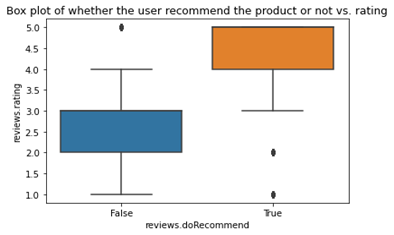
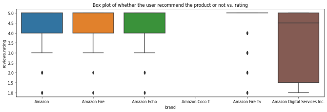
Figure 1 shows the box plot of the feature reviews.doRecommend vs. the rating of the product. We can think of the rating of the product as the polarities itself. Rating which is less than 3.0 can be considered as a negative review and ratings greater or equal to 3.0 can be taken as a positive review. Now, from figure 1, we can see that this feature clearly distinguishes the reviews as positive and negative. If the “do recommend” feature is 1 or Yes, polarity is positive and if it is No, then polarity is negative. But in figure2, we can see that the feature “Brand” is not able to separate the reviews. Clearly “Brand” does not help in identifying the polarity of reviews and hence we can discard that.
Another important point to be noted is that the reviews are given along with a timestamp. Since the timestamp is also given, the data can be considered temporal.
From the analysis and observations, we will consider only these features for the prediction
- Title of the review
- The review text
- Date of the review
- Review do recommend
Finally, we have to analyze the distribution of the output variable.
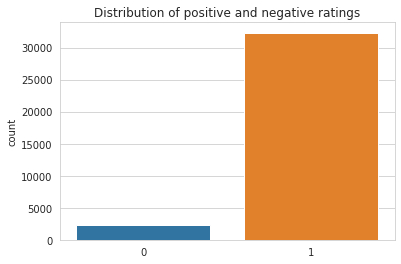
We can see that the data is heavily imbalanced because the number of negative reviews is very low as compared to the positive reviews
4.4 Text preprocessing
The preprocessing operations performed are
- Converting all letters into lower case
- Removal of stop words (except “no” and “not”)
- Expansion of words like can’t, won’t, etc.
- Removing words with length less than 2
- Remove digits and special characters
- Removing additional spaces
4.5 Feature Engineering
In addition to the available features, some new features are engineered.
- Polarity using TextBlob: We will use the text blob library to get the polarity of reviews. This will return the polarity of the review as a value in the range of [-1,1]. A negative polarity will get a polarity value close to -1 and a positive review will get a value near 1
4.6 More analysis
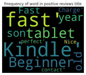
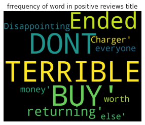
We can also analyze which all words are contributing for negative reviews and which all words are mostly seen in positive reviews. This can be done using Word Cloud. Word Cloud is a data visualization technique used for representing text data in which the size of each word indicates its frequency or importance. Significant textual data points can be highlighted using a word cloud. The visualization obtained using Word Cloud for both negative and positive reviews are:
5 Modeling
In this section, various text featurization techniques and classification algorithms are discussed. There are a total of 3 different approaches which we are going to discuss here. In all these approaches different featurization and augmentation techniques are discussed. Three models are used in all these approaches. They are:
- Logistic Regression
- Naive Bayes
- XGBoost
5.1 Approach 1 – Using TFIDF vectorizer
Here the text featurization is done using TFIDF vectorizer. TFIDF vectorization is a text featurization technique which tokenizes each word in a sentence based on two terms – Term frequency(TF) and Inverse document frequency(IDF). This is why this method is called TF-IDF. Term frequency can be thought of as the frequency of a particular word in a sentence. Inverse document frequency can be thought of as a measure of how informative a word is considering the entire corpus. IDF for a word can be written as
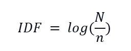
Where N is the total number of documents in the corpus (Here it will be the total number of reviews which we consider) and n is the number of documents in which that particular word is present.
TFIDF of a word will be the product of TF and IDF. We can see from the above definitions that, if a word is very common, its TF will be high, but IDF value will be very low and hence TF IDF will be low. When we use TF IDF measure, the common unimportant words will be given a low value of TF-IDF and rare but important words will be having a high value of TF-IDF.
Now that we have vectorized every sentence using TFIDF vectorizer, let us analyze the performance of this method on the validation dataset using the three models as mentioned above

We can see that performance of the models- Logistic Regression and XGboost are good and were almost similar. We can see that these models are able to classify the positive reviews with a 99% accuracy, but when it comes to negative reviews, the accuracy is poor. This is because of the heavy imbalance in the data as shown in Figure 3. Now, to solve this issue, we can try data balancing, by upsampling the negative reviews. The performance after upsampling the negative reviews are shown below.

Here we can see that the performance of models increased on the negative reviews, but we can also see the performance on positive reviews has reduced. Why?
We can see from Figure 3 that the difference in numbers between positive and negative reviews are very high. Through upsampling we are just replicating the minority class reviews without adding any extra information. Due to the heavy imbalancing, simple upsampling is not yielding very good results in this case.
But how can we solve this issue? Let me introduce you to another term- “Augmentation”. Augmentation is the process of generating more data from existing data, not by simply duplicating, but by changing and adding variations to the existing data, without changing its underlying meaning.
You can read more about nlp-augmentation here. In this case, we are using word and character level augmentations, but there are a lot of different augmentations available which can be explored. Now let us see the results after augmentation.

Here, even after augmentation, there was still class imbalance. But the performance is better than the first one and comparable to the second one. So we will be using this augmented dataset in further approaches also.
5.2 Approach 2 – Using Word2Vec
As the name suggests, word2vec is a featurization technique which is used to convert a word into a vector, or we can say to generate word embeddings. Word embedding is one of the most popular representations of document vocabulary. It is capable of capturing context of a word in a document, semantic and syntactic similarity, relation with other words, etc. Word2Vec is a technique of generating the word embeddings using a shallow neural network. You can read more about Word2Vec in this blog. Now we can apply this technique into our augmented dataset and see the results.

We can see that the performance of the models are not better than approach1 when we used word embeddings.
5.3 Approach 3 – Using BERT Embedding
BERT is a very popular neural network based technique designed for NLP tasks.
“BERT stands for Bidirectional Encoder Representations from Transformers. It is designed to pre-train deep bidirectional representations from unlabeled text by jointly conditioning on both left and right context. As a result, the pre-trained BERT model can be fine-tuned with just one additional output layer to create state-of-the-art models for a wide range of NLP tasks.”
BERT is pre-trained on a large corpus of unlabelled text including the entire Wikipedia (that’s 2,500 million words!) and Book Corpus (800 million words). Due to this incredibly large training corpus, bert is mostly used for Transfer learning purposes. BERT (Bidirectional Encoder Representations from Transformers, 2018) combines ELMO context embedding and several Transformers, plus it’s bidirectional (which was a big novelty for Transformers). The vector BERT assigns to a word is a function of the entire sentence, therefore, a word can have different vectors based on the contexts. You can read more about BERT here.
In this approach also, data is still imbalanced and augmentation is done to reduce the imbalancing problem.

We can see that using BERT has achieved very good results when compared to the other two approaches without the data balancing.
6. Conclusion
In this article, I have explained about sentiment analysis which is a very useful and important task in NLP. I explained about the dataset, feature analysis, data cleaning and pre processing, feature engineering and visualization. I tried to discuss various featurization techniques for sentence classification tasks. Three different techniques – TFIDF, Word2vec and the BERT were discussed in this article.
I hope you enjoyed the blog. In case of any queries or suggestions, please feel to contact me through LinkedIn. You can also checkout my Github repository here.
