
In this article we will talk about two parts of Mathematics which are used in Machine Learning. 1) Coordinate Geometry and 2) Calculus.
But before discussing that, Let us start from a very basic question. What we try to do when we build a model. We try to predict something, right? Once our model predicts the outcome, we compare it with the actual observations. By comparing this predicted value with actual observation, we identify how good our model is.
Now, let’s ask another question. What is that calculation through which we see how good our model is performing? The error, right? Calculate the difference between the actual value and predicted value and call it error.
Now, if our error is huge, we try to reduce the error by modifying the model. So, our ultimate goal is to reduce the error. One of the uses of Calculus is to find a point where a function achieves minimum. That is what we want. We want a point where error function achieves minimum value (if you are not clear what is minimum value, it is explained below) , and that is the point where our model will perform best.
This is one of the applications of mathematics in Machine Learning. There are many more applications of mathematics (Probability, linear algebra, statistics etc) that I will discuss in further articles. Lets understand the use of calculus in finding the minimum of a function.
Here we will discuss two parts of mathematics, 1) Co-ordinate Geometry 2) Differentiation (part of Calculus)
Let us start with co-ordinate geometry. In co-ordinate geometry any point is indicated by its x position and y position.
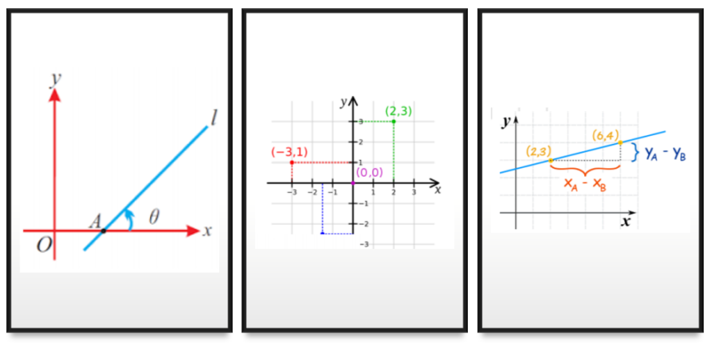
In this image, one point is indicated by (0,0). That point is called origin. Any other point e.g. (2,3) is 2 unit away from origin on x-axis and 3 unit away from origin on y-axis. Similarly, a point (x,y) is x unit away from origin on x-axis and y unit away from origin on y-axis.
Any two points on x-y plane can make a line. In the next figure, (2,3) is one point and (6,4) is another point. So, these two points can make a line as shown in the figure.
Now, the next concept comes the inclination of line with xaxis, this is called slope. To measure the slope, you have to start from x-axis and reach to the line in anticlock wise direction as shown in the figure. Slope is defined as tanθ, which is nothing but Rise/Run. Now, rise = (Ya-Yb) = (4-3)=1 and run = (Xa-Xb) = (6-2) = 4. So, slope = Rise/Run = ¼ . Now, if some line is parallel to x-axis then, its rise will be 0. Hence, slope = 0/run = 0. Hence, if a line is parallel to x-axis then its slope will be 0.
Any line is given by equation y= (slope * x) +Intercept. I am discussing this because it has extensive use in Machine Learning.
Now, coming to calculus part, Many of you must have seen that we use dy/dx . This dy/dx is called differentiation and this is nothing but the slope of a line that is drawn on a function at any point. Meaning dy/dx = slope = Rise/Run = (Ya – Yb)/(Xa – Xb).
Let us say, our line is y = slope*x + intercept ; y = 3x+ 4, then the slope of our function y is 3 and intercept is 4. Hence, from the definition dy/dx of function y = 3.
You can understand for simplicity it is nothing but the difference between y divided by difference between x.
Let us understand some function, We have described the equation of line above as y = (Slope * x)+ Intercept . This is nothing but a function of y in x. y = 3x+4 is function of y in x of degree 1, because x has power 1. y = 5x2 + 5x+9 is another function of y with degree 2 as the highest power of x is 2. Y= 5*x2 +9 is again a function of y in x with degree 2, because the highest power of x in this function is 2. So, if anyone is writing y = f(x), it means it is function of y in x with some degree. Our function can be of any variables. Example, z = 3x+4y or w = z2+7x+8y3. Now let us understand one more concept of tangent. A line on any point of a curve which is just touching the curve is called tangent.
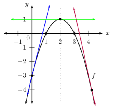
In this graph, we can see there are three tangents drawn on function f. One is red line at bold dot, one is blue line at (0,-3) point and one is green line which is parallel to x-axis. It is to note here, if a line is parallel to x-axis, then it is indicating either the maximum point or minimum point on the curve. Meaning, to find a minimum point on the curve, you have to find the line which is parallel to x-axis i.e. its slope is “0”. If you remember, I explained earlier, slope is dy/dx = differentiation. Hence, to find the minimum point of a function y = f(x); we have to find dy/dx for y and then we have to equate dy/dx to 0. i.e. dy/dx = 0. By solving this we can find the point where the function achieves minimum. Note: for more than one independent variables, we use partial differentiation. This we will discuss in next reading.
Now, imaging, we have error function y = f(x). Our aim is to minimize this function so that we can get the best model. Now, we are differentiating this function as dy/dx, and equating it to 0 as dy/dx = 0. This will give us some x value, and y-value. By putting those values in y= f(x) will fetch us minimum value of error, which is the desired result.
Now, Suppose our error function of the model that we have build is y= 5x2 + 5x+1. Try to sketch the graph of y= 5x2 + 5x+1. It is shown in the next graph.
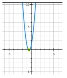
The yellow dot is the minimum point. To find that point, we have to calculate dy/dx for
the error function and then, dy/dx = 0. Just for the reference, the dy/dx for y is 10x+5.
If we equate this dy/dx to 0, then 10x + 5 = 0, so x = -5/10 = -0.5. By putting this value
of x in error function, we can get the error value y. We use this method in linear
regression to calculate β0 , β1 etc.
For the reference, here is the list of some function and its dy/dx:
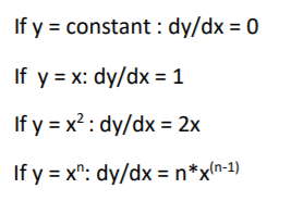
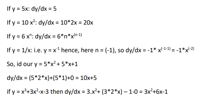
I am giving some examples for practice, I would suggest to practice on these problems.
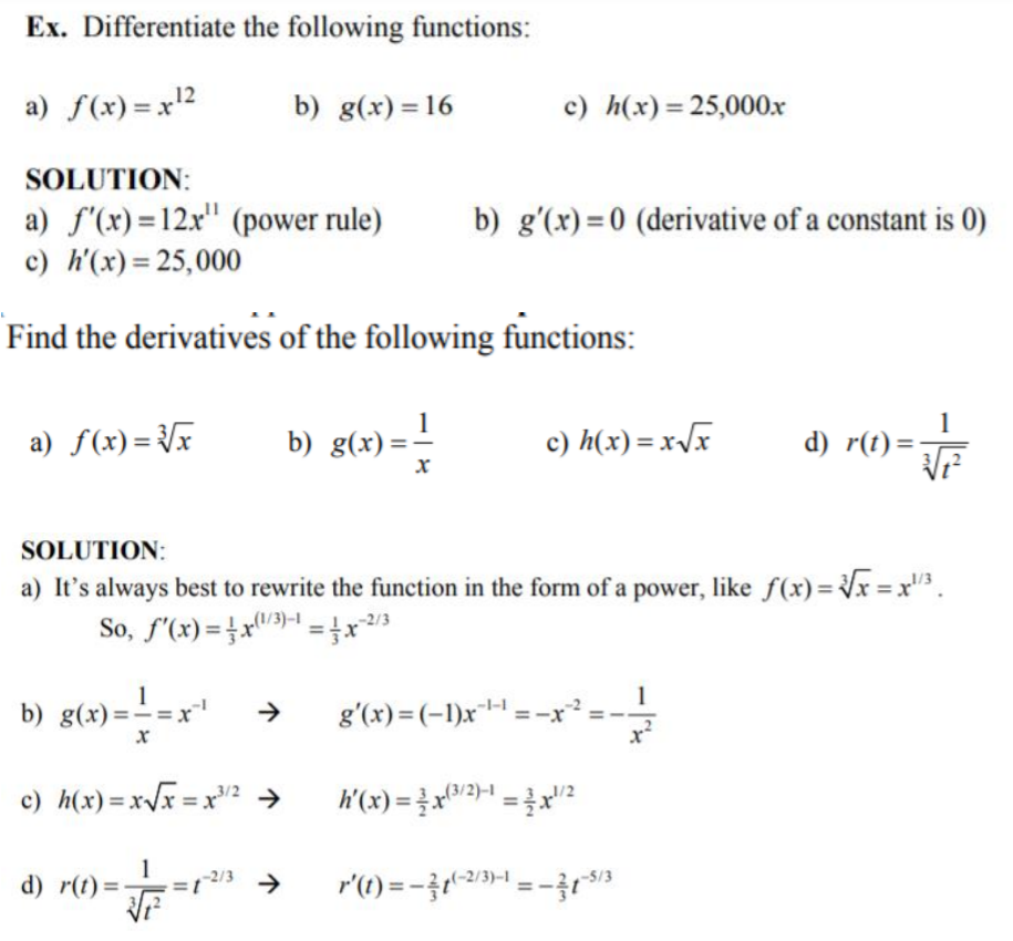
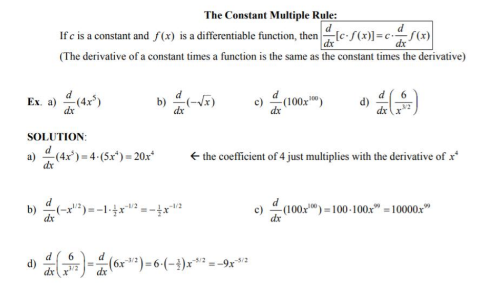
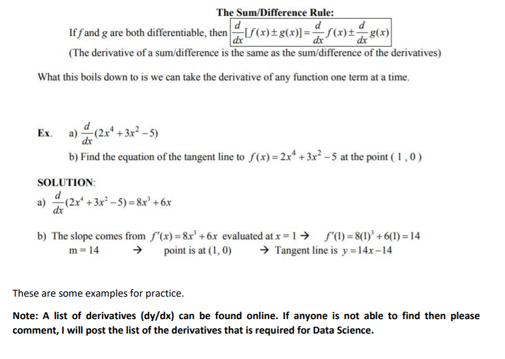
I hope this is clear. I am trying to explain the mathematics used for Data Science in this reading, this is used in machine learning in very extensive way. But, it is very important to understand the basics, How those calculations are performed. Now, use this concept and List square method to find the coefficient of linear regression coefficient (give it a try). I would suggest to do a lot of practice on these concepts. I will post next reading in which I will explain the partial derivative (partial differentiation) and apply differentiation to calculate the coefficient of linear regression. Any comment or suggestion to improve the reading is highly appreciated.
[Reference]: http://www.pstcc.edu/facstaff/jwlamb/1910/1910_3_1.pdf
