Mathematics for Machine Learning

Probability Theory

NOTE: This blog contains very basic concepts of probability

Probability is used in many parts of Machine Learning. Hence, it is very important to understand this topic very carefully. There are different terms that should be understood before understanding the concept of probability. Let us discuss these terms:

1) Random Experiment : let us say we are playing a board game and we throw dice. The manner of throwing dice is same every time, but we get different number every time. Some time we get 1 or 2 or any number between 1 and 6. This activity is called random experiment. The experiment we are doing in same manner every time but we are not getting same result every time. An experiment that can result in different outcomes, even though it is repeated in the same manner every time, is called a random experiment.

2) Sample Space : when we throw dice we get any number between 1 to 6. So, set of all possible numbers together forms Sample space. In this case, sample space = {1,2,3,4,5,6)
The set of all possible outcomes of a random experiment is called the sample space of the experiment. The sample space is denoted as S.

3) Discrete and Continuous : Let us understand in a very basic form. When you have to jump to go from one point to other point there is no path, then it is discrete. But when there is a road between two points and you don’t have to jump then that is continuous. So, discrete is countable but continuous is not countable. There can be infinite number of points between two point in continuous. In Discrete, we do not consider those points and we are concern with only two point on which we are jumping. A sample space is discrete if it consists of a finite or countable infinite set of outcomes. A sample space is continuous if it contains an interval (either finite or infinite) of real numbers.

4) Event : one outcome of any sample space is event. Like getting 1 in throwing a dice is one event similarly getting 2 in throwing a dice is another event. So, in our dice example there are six event. Each outcome is one event. An event is a subset of the sample space of a random experiment.

5) Now suppose we have two dice, one is blue dice and another is red dice. Getting 1 on each dice is one event. Getting 1 on blue dice and 4 on the red dice another event.
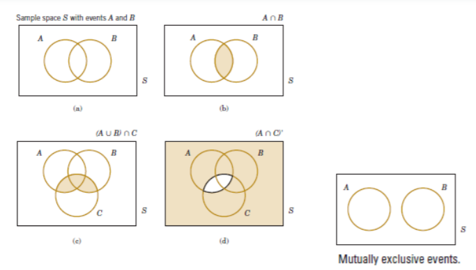
• The union of two events is the event that consists of all outcomes that are contained in either of the two events. We denote the union as E1 ∪E2.
• The intersection of two events is the event that consists of all outcomes that are contained
in both of the two events. We denote the intersection as E1 ∩E2.

• The complement of an event in a sample space is the set of outcomes in the sample space that are not in the event. We denote the complement of the event E as E′. The notation EC is also used in other literature to denote the complement. Suppose we have two dice, one is Blue and other is Red. We are throwing both the dice and we want 1 on each one. So there are four different possible outcome. Either both have 1 or both have any number but not 1 or blue has 1 and red does not have 1 or red has 1 but blue does not have 1. So out sample space will be S = {11, 1n,n1,nn}

Let Subset of Sample-space is at least one 1 on any of the dice E1 = {11,1n,n1}
Hence E1’ = Compliment of E1 = {nn}
Let another subset is at least one dice has no 1 on it E2 = {1n,n1,nn}
So E2’ = {11}
E1 ∪E2 = {11,1n,n1} ∪ {1n,n1,nn} = we will take all possibilities that are present in both E1 and E2 = {11,1n,n1,nn}
E1 ∩E2 = {11,1n,n1} ∩ {1n,n1,nn} = We will count only the common one = {1n,n1} as only these two are present on both E1 and E2.

6) Mutually Exclusive : If nothing is common in between two event then it is called mutually exclusive events.
Two events, denoted as E1 and E2, such that E1 ∩E2 = φ are said to be mutually exclusive. Φ means nothing is common between E1 and E2.
I am taking an example from Book for better understanding. The book detail is given in the reference.

7) Factorial: It is denoted by !, eg n! is n-factorial. How it is calculated?
Let us take some example:

1! = 1 = 1
2! = 2 x 1 = 2
3! = 3 x 2 x 1 = 6
4! = 4 x 3 x 2 x 1 = 24
5! = 5 x 4 x 3 x 2 x 1 = 120
I hope it is clear now. One thing to note here is 0! = 1

Permutation: Consider a set of elements, such as S = {a,b,c}. A permutation of the elements is an
ordered sequence of the elements. For example, abc, acb, bac, bca, cab, and cba are all of
the permutations of the elements of S.
The number of permutations of n different elements is n! where
The number of permutations of subsets of r elements selected from a set of n different elements is
= n! / (n-r)!
It is denoted by :

One important formula to note here is:

Combination:

After understanding these few concepts, lets start the probability theory:

Let us understand probability from a basic example. If we are tossing a coin, what outcomes can come? Either Head or Tail. If coin is unbiased meaning chances of head or tail are equal, then we calculate the probability of tail as follows:

What is the total sample space?
{Tail, Head} = 2 right? (meaning there can be two outcomes possible)

What we want to calculate?
Tail = 1 (meaning we are interested in only one outcome)
So, P(Tail) = (We are interested in the outcome)/ (Total possible Outcome) = ½

Similarly, P(Head) = (we are interested in head)/(Total possible outcome) = ½
Let us take another example, We are throwing a dice, we want to calculate the probability that a number that comes on the dice which is less than 3. Hence, what is the total possible outcome? {1,2,3,4,5,6} = 6 (total possible outcome}

We are interested in {1,2} = 2 (two possible outcome)

Hence P(x<3) = we are interested in/total possible = 2/6 = 1/3

If we are interested in P(x>= 3) then

Total outcome we are interested in {3,4,5,6} = 4 (4possible outcome) P(x>=3) = 4/6 = 2/3

Note: probability will always be in between 0 and 1, probability can not go below 0 and can not exceed 1.

Another example, if we are throwing two dice, we are interested in the numbers showing on the dices, the sum of which should be 4.

So, total possible outcome =
{(11),(12),(13),(14),(15),(16),(21),(22),(23),(24),(25),(26),
(31),(32),(33),(34),(35),(36),(41),(42),(43),(44),(45),(46),
(51),(52),(53),(54),(55),(56),(61),(62),(63),(64),(65),(66)} = 36

Here (11) meaning first dice show 1 and second show 1
(2,3) meaning first dice show 2 and second show 3 and so on

We are interested in = {(13),(31),(22)} = The sum of the numbers showing on dice 1 and dice 2 should be 4 = 3
Hence, required probability = P(x=4) = We are interested in/total possible outcome = 3/36 = 1/12

Few Things:

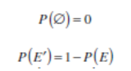
It means, probability of head in a coin P(E)= ½
Then probability of Tail in a coin P(E’) = 1 – P(E) = 1- (1/2) = ½

If P(x<3) = P(E) = 2/6 = 1/3 Then P(x>=3) = P(E’) = 1- P(E) = 1-(1/3) = 2/3 which we got above.

There are some rules in probability. We have discussed Union and intersection above, if two event A and B are there, then

P(A union B) = P(A) + P(B) – P(A intersection B)
If A and B are mutually exclusive event, i.e. nothing is common between A and B, then

P(A union B) = P(A) + P(B)

As P(A intersection B) will become 0 (zero).

One more thing, what is equally likely events, when chances of every event to occur is same then the events is called equally like events. Example, in tossing a coin, chance of getting a head is same as chance of getting a tail. So both the event is equally likely event.

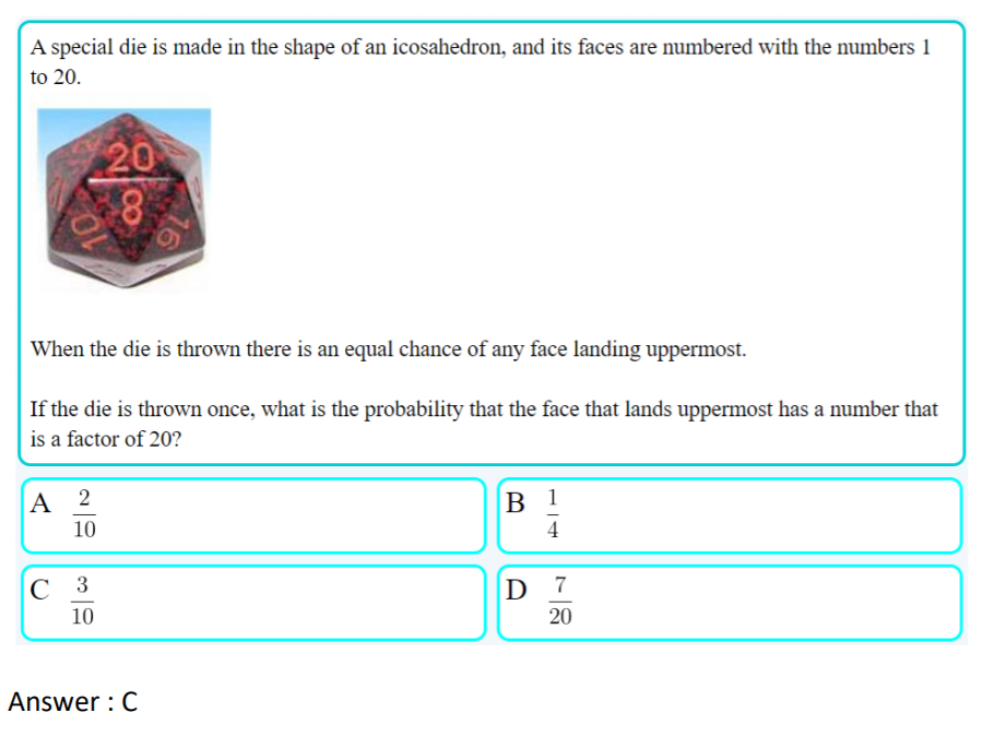
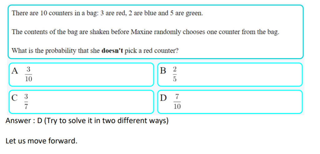
Try to solve a question:

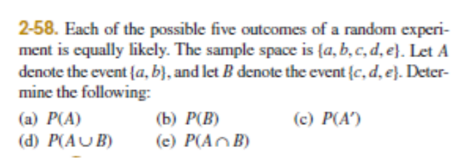
Approach to solve a problem may be always find the sample space and then find the event in which we are interested. Another question is there

I am taking these questions from the book, the detail description of the book is provided in reference. Readers can solve many more question, as the book is providing a number of questions. If reader find any difficulty in solving these problem, please let me know, I will try to explain further.

Question:

Conditional Probability:
Let us understand this with one example. Suppose we have tossed the coin once and we got head. Now, what is the probability of getting head again if we toss the coin next time. This is called a conditional probability.

We want to calculate the probability of an event, knowing the probability of previous event. Conditional probability is denoted by P(B|A), this means we want to calculate the probability of B, also we the probability of event A already.

Note: if the event A and B are independent, then conditional probability of event B, give the probability of event A is simply the probability of event B P(B).

In our coin example, every time tossing of the coin is independent of the previous tossing. Hence, every event is independent in this case. Hence, Suppose we have tossed the coin once and we got head. Now what is the probability of getting head again if we toss the coin next time? It will be P(head) = ½

Conditional probability formula is

P(B|A) = P(A and B)/P(A)

Let us take one more example:

We have one bag in which 5 green and 8 yellow balls are there. What is the probability of getting a green ball?

P(x=green) = what we want/Total possible outcome

We want green, which can be any one of 5 green balls. Total possible outcome is either green or yellow ball, which is any one of (5+8) = 13 balls.

Hence, Probability (x= green) = 5/13

Now, if we want to pick one more time, saying in the first time we got a green ball, this time no. of green balls is 4 and total number of balls are (4+8) = 12.

Hence, the probability of green ball is P(x= green) = 4/12
What is we had yellow ball in the first selection? The bag still contains 5 green ball and no. of yellow ball is 7 now. Hence, P(x=green) = 5/(5+7) = 5/12

Hence, Second probability depends on the first probability.

If we will put the ball back in the bag after first trial, then result will not change. Hence in that case, next probability will not depend the previous result. Isn’t it obvious. We took one ball from bag, and before doing the next pick, we put the ball back in the bag. Hence nothing changed. This is called Replacement.

I found some example which will be good to do practice:

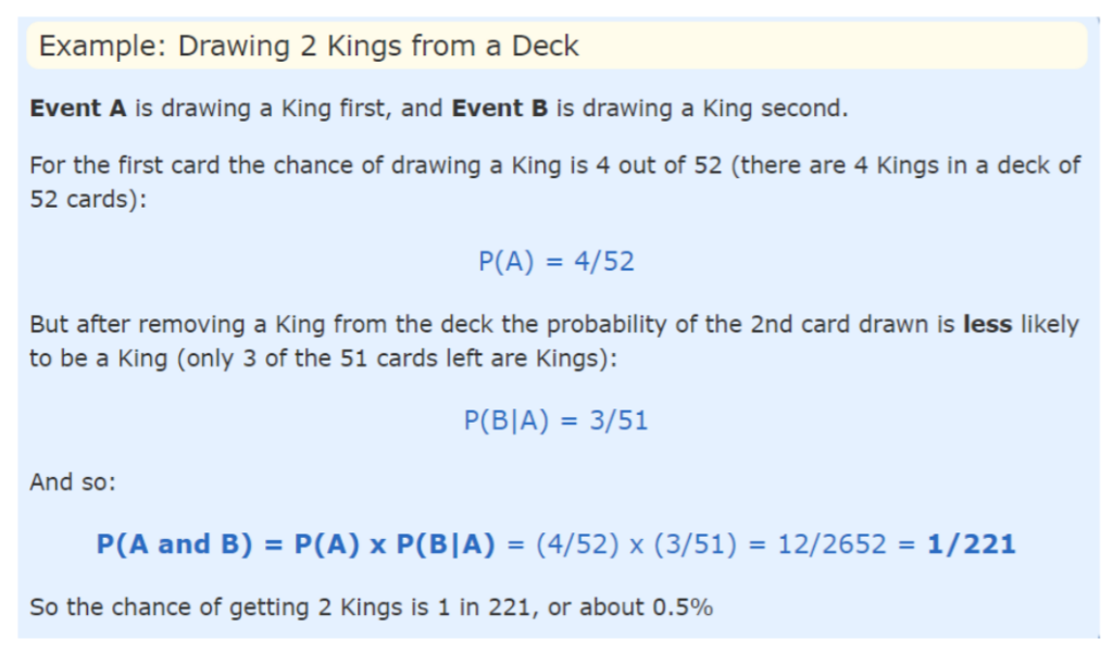
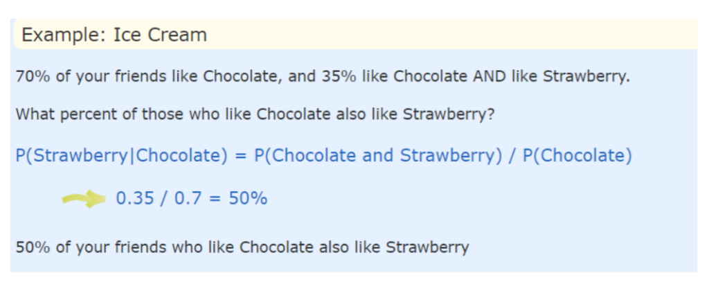
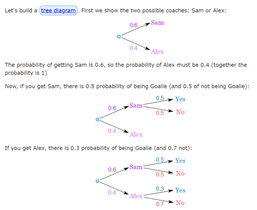
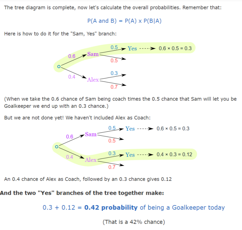
Please do some problems on conditional probability. The book and the website from which some contents has been taken for this article is mentioned in the reference.

Note: One thing to note here is P(A and B) = P(A ∩ B) = P(B ∩ A)

Hence, P(B|A) = P(A ∩ B)/P(A)

Bayes’ Theorem :

Let us take one mathematical calculation here:

P(A|B) = P(A ∩ B)/P(B)

i.e. P (A ∩ B) = P(A|B) P(B)

Also, P(B|A) = P(B ∩ A)/P(A)

i.e. P(B ∩ A) = P(B|A) P(A)

as we know P (A ∩ B) = P (B ∩ A)

Hence, P(A|B) P(B) = P(B|A) P(A)

This is called Bayes’ Theorem.

If we know the probability of two events A and B and conditional probability of A with respect to B, then we can calculate the conditional probability of B with respect to A.

We should note here, if we are calculating P(A|B)= P(B|A) P(A)/P(B), then P(B) > 0 we can not divide anything with zero. This is meaning less (many people say it is infinity, but no it is meaning less and not infinity, as infinity has meaning and carries a considerable significance in Mathematics world).

Please do a lot of practice on Conditional Probability and Bayes’ Theorem. Because Bayesian
Statistics, Random Walk, Markov Chain, Monte Carlo Simulation and many more have
extensive use of Conditional Probability and Bayes’ Theorem. Above mentioned concepts will
be discussed in further readings.
Next, I will discuss the probability distributions

Reference:
1) https://www.mathsisfun.com/data/probability-events-conditional.html
2) Applied Statistics and Probability for Engineers By Douglas C. Montgomery and George C. Runger