Transformer models has become the go-to model in most of the NLP tasks. Many transformer-based models like BERT, ROBERTa, GPT series, etc are considered as the state-of-the-art models in NLP. While NLP is overwhelming with all these models, Transformers are gaining popularity in Computer vision also. Transformers are now used for recognizing and constructing images, image encoding, and many more. While transformer models are taking over the AI field, it is also important to have a low-level understanding of these models. This blog aims to give an understanding of Transformer and Transformer based models. This includes the model components, training details, metrics and loss function, performance, etc.
Pre-requisites
- Embeddings
- Sequence modeling
- RNNs and LSTMs
Pre-requisites
- Embeddings
- Sequence modeling
- RNNs and LSTMs
A little background
Nowadays, neural network-based models are gaining popularity in the field of computer vision and natural language processing (NLP). But back in the early 2000s, NLP was not very much popular and the fun in AI was happening in computer vision alone. Computer vision was gaining popularity back then through the ImageNet challenge and models like AlexNet, ResNet, GANs, etc. were catching the headlines. Computer vision was so attractive that NLP was not much in the picture.
However, at the same time, NLP was also making some progress through models like Word2Vec. Word2Vec is a Neural network model invented by Google in the year 2013. This model can generate context-independent embeddings to text data. Word2Vec models were a key breakthrough in the field of NLP because this was one of the first models that could generate embeddings based on the semantic meaning of a word.
However, this was not enough. One basic disadvantage of the conventional neural networks was their inability to memorize things. This was really important in sequence to sequence applications like machine translation, image captioning, etc. This disadvantage was however overcome by the popular Recurrent Neural Networks (RNN) in the year of 2014-2015. Again the RNN model also put forward many challenges like vanishing gradients, exploding gradients, handling long-term dependencies, etc.
This was later solved by another model series known as LSTMs. LSTM models were originally invented in 1997, but they gained popularity after the invention of RNNs. LSTMs can be considered a great advent in the field of NLP. LSTMs can handle vanishing/exploding gradient problems, memorize things in a more smart way. There are other variations in LSTMs also, which are still widely used by many companies. These include bidirectional LSTM, GRUs, and many more. If you like to read more about LSTMs, I recommend you to check out my previous blog post.
It was in the year 2017, the NLP made the key breakthrough. Google released a research paper “Attention is All you need” which introduced a concept called Attention. Attention helps us to focus only on the required features instead of focusing on all features. Attention mechanism led to the development of the Transformer and Transformer-based models.
Why Transformers
LTMs were great. But there were a few limitations also. The first one was that LSTMs was difficult to train. This is mainly because of the longer training time and also the high memory requirements during the training. LSTMs were mainly used to overcome the vanishing/exploding gradient problems by RNNs. But it turns out that LSTMs solve this problem only to a certain extent. Another disadvantage of LSTM is that it can easily overfit and it is very difficult to include regularization techniques. So now we came to know that LSTMs cannot rescue us completely from all these issues. So what now?
Here comes the Transformers. The invention of Transformers can be considered as the “BAM” moment of NLP. So what extra benefit does Transformer offer? Let’s first have a high-level overview of Transformers, and then we can deep dive into its components and their working in the following sessions
Transformers
At a very high level, Transformers can be considered as an Encoder-Decoder model, where the Encoder will take our inputs and convert it to a vector. These encoded inputs are given to the Decoder, where the Decoder tries to convert the vector into a Natural language, or an interpretable language. Now, if we think about the above process, we can relate it to machine translation (eg: converting a French sentence to English) or image captioning (generating captions for images). When we use a Transformer for machine translation, we give our input sentence (a French sentence) to the encoder. The encoder will convert the text into a vector. Now, this vector is passed to the decoder, where it converts it to an English sentence. The same method applies to image captioning also, where the input will be an image and the output will be a sentence that describes the image.
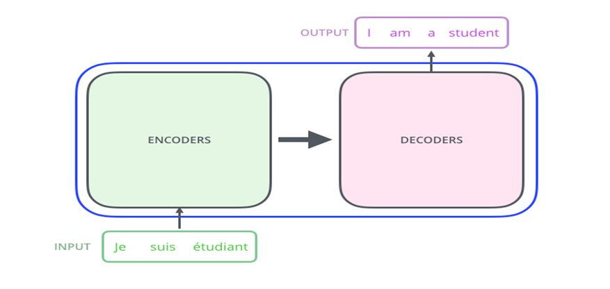
Now, the Encoder and decoder blocks are actually a stack of encoders and decoders as shown in the figure. The input goes to the first encoder stack. It will convert the input to another vector Z, then this vector is passed to the next component and so on. The output from the final encoder layer will be given to the decoder stack. All the encoders have a similar structure and similar layers in them, except that the weights are different and are learned during the training process. Similarly the decoders are also having the similar structure.
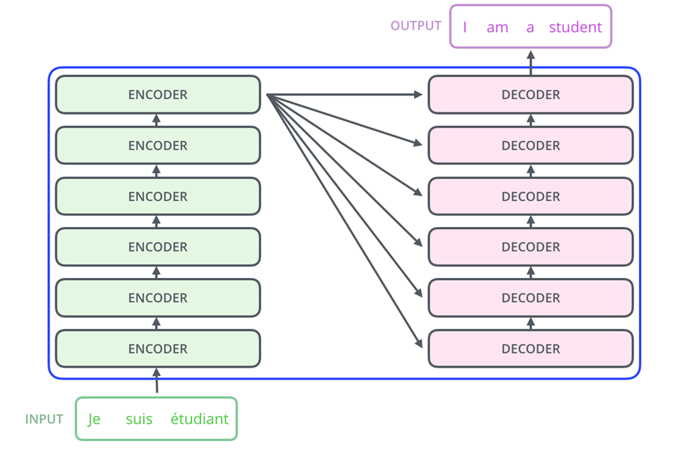
All these are fine. But what is so special about Transformers when compared to the previous models?
- Transformers can handle long-term dependencies better than LSTM
- Solves the problem with vanishing/exploding gradients
- Encoding is Bidirectional
- Supports parallelization
Each of these benefits will become more clear as we go forward.
Encoder Stack
Since all the encoder stacks are similar, we will be taking a single encoder module for understanding the same. Now, an encoder needs to encode our input. While encoding it needs to make sure that the Decoder module gets all the relevant information to Decode. Now how does it work? Let’s have a look into the encoder structure.
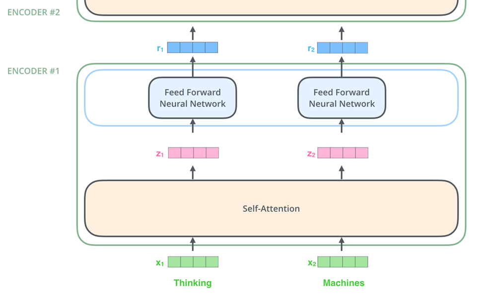
From the above figure, we can see that one encoder unit contains two blocks- Self attention block and Feed forward neural network. I am assuming you are already familiar with the feed forward neural network, so I wont be explaining that. Let us focus on the Self-attention layer.
Self-Attention Layer
If you remember in RNNs and LSTMs, for generating the current hidden state, we require some memory about the previous events. Getting the information from the past or the future events is very important, because it helps us to get the context and this in turn will make the prediction more accurate. In the Transformer encoder the idea is similar, but with some changes.
In encoder we are giving our input sentence splitted into the words. Now from Figure 3, we can see that each word is converted into a vector. Now while generating these vectors, wouldn’t it be great if we could get the context also. A similar process happens through Self-Attention layer
For example, consider a sentence
“The animal didn’t cross the street because it was too tired”
Now imagine we need to translate this sentence. For that, first we need to encode it. Now while encoding we pass all the words in this sentence to the encoder (all at the same time). Now while we start the encoding we came to know that, for encoding some words, some context is also required. For example, the word “it” – whether it refers to the animal or the street. Now, this is where we use the self-attention mechanism. In the end we will get an attention matrix which contains how each word is important in encoding a particular word. The attention matrix for the above example will look something like this. The darker the cell is, the more attention will be required.
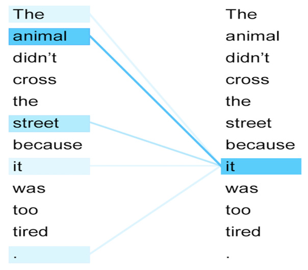
Now, once we get the attention matrix, the next step is to calculate the vector Z. Now this Z will be the encoded vector representation of each word. Now how this vector is actually calculated?
Attention Matrix and Encoded Vector – Z
The first step, we need to do with our input (already embedded as vectors), is to calculate the attention matrix. We already know what the Attention matrix is, now lets see how it is calculated.
Attention Matrix
The Attention Matrix is calculated using two vectors – Query and Key. There is another vector called value vector, which is used in the later stage. For every word in our input sentence, there will be a query, key and value vectors. Now these vectors are calculated by multiplying the input word (the embedding) with a matrix, as shown below
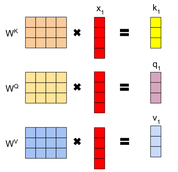
As shown in the above figure, each of the input word vectors (x1 in the figure) is multiplied with some matrices to generate the key, query and value vectors. The matrix used for multiplication is learned through backpropagation. Let’s assume we have fixed the input dimension (number of input words) as L, and the dimension of the weight matrices be dxd. When we compute these vectors for all the input words, the dimension of these vectors will be 1xd. Now when we concatenate all these vectors for all the input words, the resultant vector will be Lxd.
Okay, so now we got these three vectors. How do we now compute the attention matrix? Once we get these vectors, the attention matrix is calculated as:
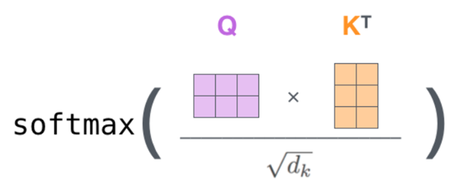
The final softmax layer is to ensure that the attention matrix will contain values in the range of 0-1. A value indicating the high importance of a word in encoding the current input word. The attention matrix will be of order LxL
Now the next step is to calculate the vector z. This vector is calculated by multiplying the value vector with the Attention Matrix. So, this will result in a vector which is Lxd dimension, which indicates the L number of vectors having a dimension of d. The overall process of calculating the z-vector can be shown as shown below:
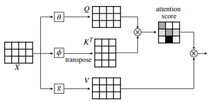
While encoding a particular word, the query, key and value vectors will help us to focus more on the important words (based on the attention weights) and take little or no information from the irrelevant words. Now these vectors are passed to the next encoder unit and the same process repeats.
Now it is the time to see how one complete encoder unit will look like
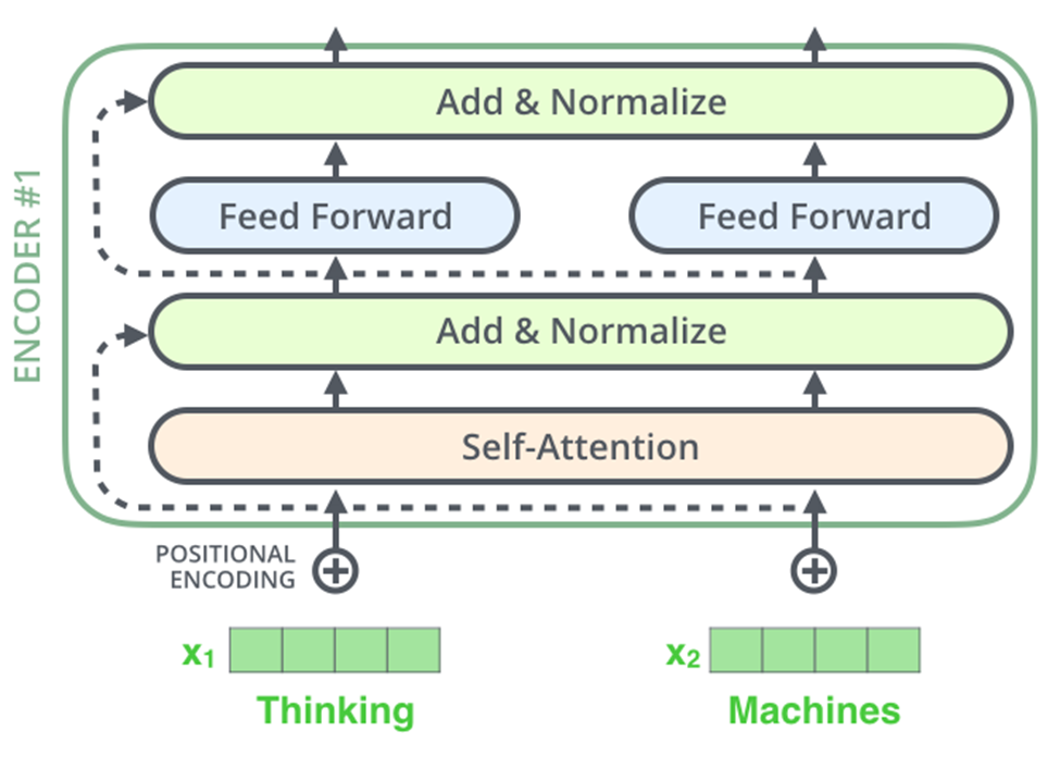
We can see some more terms here
- Positional encoding – This is a way to indicate the position of a word in a sentence
- Normalization layer – Layer normalization will normalize the distribution of each layer output
- Residual connections – The residual or skip connections will prevent the vanishing/exploding gradient problems and also prevents the chances of overfitting
Decoder Stack
Now that we understand the encoder architecture and how it works, it will be very easy to understand the decoder part of the model.

From the above figure, we can see that the encoder and decoder are very similar with an extra unit on the decoder side. This is Encoder-Decoder attention. Lets understand the attention mechanism from the Decoder’s view
- Self attention – This works similar to that in Encoder. But there is a little difference here.If you remember, the self attention in the encoder, for the current word, we have to consider the key, value and query vectors corresponding to all the words. That means, the current word has to consider the past as well as future words for attention, which makes this process a bidirectional one. But the function of the decoder is to predict the next word. So, while computing the attention vector for the current word, we can only consider the past words, because the future word is not yet known to us and it is to be predicted. This makes the decoder attention process unidirectional
- Encoder-Decoder attention – This layer will compute the attention between encoder and decoder and tell us how important each encoder vector component is in predicting the next word.
Output Layer
The final part of the model is to get the outputs in the required format. For example, if the task is machine translation, then the output should be a sentence in the required language like English or French. Now how do we get the output as words or sentences?
Let us assume, in our task, the target language is English and we have a total of 1000 words in our vocabulary. Now, the final output layer in the Transformer model is a softmax layer of size equal to the size of the vocabulary. The output will be values from 0 to 1 which are actually the probability of each word as output. For example, if at time t=1, the output vector is like this
| Am | I | The | Student | Van |
| 0.9 | 0.05 | 0 | 0.01 | 0.04 |
Then the output word at t=1, will be “am”. Like this, each output word will be predicted until the <EOS> condition is reached.
Training details
Transformers are trained on huge amounts of data. The training is done through the Backpropagation algorithm and the loss functions used were cross entropy loss and Kullback-Leibler divergence.
Transformer variations
Even though the transformer can be considered as a big “eureka” moment for all NLP engineers, it also comes with some challenges. The self attention mechanism in the transformer itself has the problems associated with quadratic memory and quadratic computation time requirements. Some other similar architectures were also introduced to mitigate these issues, including Sparse Transformers, Longformers, Performers, etc.
Final thoughts
I hope you enjoyed the article. This blog tries to cover a basic overview of transformers, and its architecture. However, I have also skipped some details like Multihead attention, positional encoding etc., and I strongly recommend you to read more about the same.
For any queries or suggestions, please feel to contact me through LinkedIn or Twitter
