Overfitting is one of the major problems while training our machine learning models. Overfitting means it is capturing each data point accurately in the training dataset which can result into the model’s inaccurate or low performance on an unseen dataset. This can easily be understood through below graph:

As we move to the right in the above graph, we can observe that, the curve is trying to capture each point of observation. Hence, it seems that the model tries to learn too well the details and causing overfitting which will result in poor performance on testing data.
Regularization is one of the methods which helps to reduce the overfitting while modifying the learning algorithm slightly. In the Linear Regression algorithm, it penalizes the coefficients, in Deep Learning it penalizes the weight metrics of the nodes. In order to understand the modifications done to the algorithm, we are taking the Linear Regression algorithm so that it will be easy to understand the regularization method.
The linear regression equation looks like this:

Here, Y is the dependent variable and the Xs are independent variables and β is the coefficient of each of the X variables of the regression equation. One of the methods to determine the coefficient/parameter values is the Ordinary Least Square (OLS) method which minimizes the sum of squared errors or cost function. This means that given a regression line through the data, we calculate the distance from each data point to the regression line, square it, and sum it, and sum all the squared errors together. This is the quantity, that is also called as cost function, that ordinary OLS seeks to minimize.
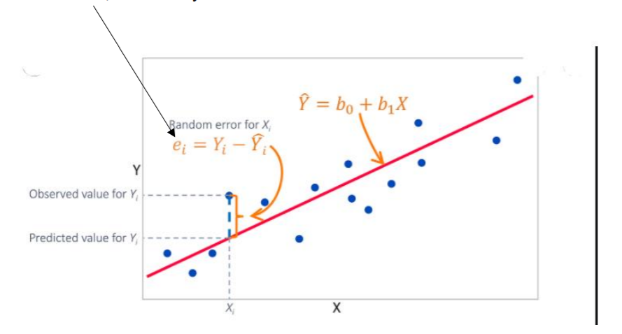
OLS treats the data as a matrix and uses linear algebra operations to estimate the optimal values for the coefficients. However, sometimes training the model with this method result into increased complexity as the training model learns each of the data point and causes overfitting and does not generalize well to the future dataset. In order to reduce this complexity of the model or overfitting while minimizing the sum of square error, we use regularization methods, where it adds penalty terms to the cost function to get the best fit line. The two types of regularization methods are explained below:
1) Lasso Regression/ L1 Regression: First, we will know that why it is called as L1 regression.
It uses first order penalty to the loss function hence called as L1 regularization. We all know the cost function which is sum of the square of errors in case of linear regression algorithm.

In Lasso, we add penalty term λ x | the slope | ,where Lambda λ is a tuning parameter that decides how much we want to penalize the flexibility of our model. Now the equation looks like:
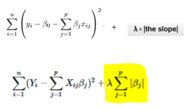
Now let’s suppose due to overfitting there is no difference in actual and the predicted in training data, hence,

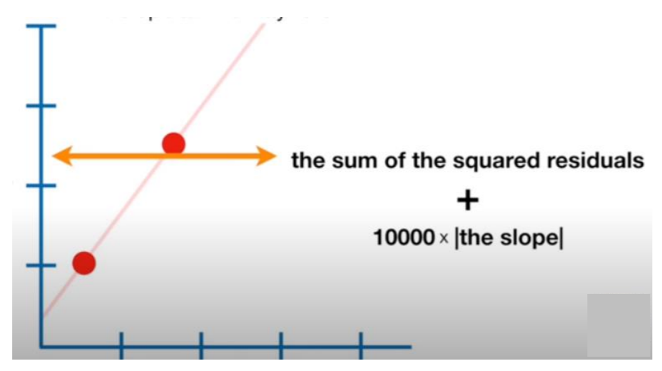
Now let’s take λ = 1 then the absolute sum of slope that is β1 + β2 + β3 …. , will have some value which will be added to this zero then the total cost function value will be more than zero which will result in deviating the best fit line a little bit from the actual data points and reduce the overfitting. As stated, that λ is a tuning parameter so as it will increase the slope which is coefficient can shrink all the way to zero as shown in the below image.
This process of tuning the λ can help in variable reduction. As for example,
Y = βo + β1X1 + β2X2 + β3X3 + ……. + βnXn
to minimize the loss function with respect to each coefficient of the equation above, we take the derivative of loss function with respect to each individual coefficient and equate it to zero (Slope of the tangent line of the curve at that point should be zero, see figure below).
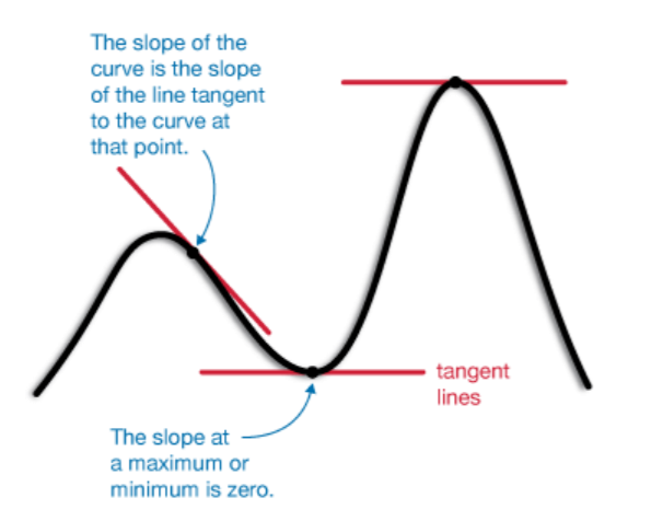
β1new = β1 – η[δL1 /δ β1] (With this equation through which we update the weights or coefficient of the equation, η is a constant). If by solving the above equation, β1 shrinks to zero then β1X1= 0, hence X1 can be removed which will help in reducing the complexity of the model (Complexity is the number of features in the model, less number of features, less complex the model is). Now the question is how we decide the value of λ, we just try a bunch of values for λ and uses Cross-Validation, typically 10-fold Cross-Validation, to determine which one results in the lowest variance.
1) Ridge Regression/ L2 Regression: So now you must know why it is called L2 regression.
Yes, this is because it adds a second-order penalty in the loss function. There is not much difference in the algorithm, it uses the square of the slope of the regression equation.

Now the coefficients are estimated by minimizing this function. Again, λ here is the tuning
parameter which decides the flexibility of the model.
The key difference between both these techniques is that Lasso shrinks the less important feature’s coefficient to zero thus removing some features all together. So, this works well for feature selection in case we have a huge number of features. While Ridge regression make favors the smaller parameter values as it does not turn the coefficient to completely zero. Hence, when sample size is relatively small, then Ridge regression can improve the prediction made from new data by making predictions less sensitive to the Training Data. The Ridge regression penalty is λ times the sum of all the squared parameter except for the y-intercept. Let us understand with an example of first coefficient of regression equation. If we do the LASSO, in penalty term, derivative of β1 (δL1/δβ1 = δ((y – predicted) 2+ λβ1 + λβ2)/δβ1 = δ((y – predicted) 2 / δβ1 + λ δβ1/ δβ1 = δ((y – ypredicted) 2 / δβ1 + 0) becomes 0. But, in Ridge, the penalty term is square, hence the derivative will be 2λβ1 (δL1/δβ1 = δ((y – ypredicted)
2+ λβ1 2 + λβ22)/δβ1 = δ((y – ypredicted)2/ δβ1 + λ δβ12/ δβ1 = δ((y – ypredicted) 2
/ δβ1 + 2λβ1 ),
which is not zero. Hence, it penalizes the weight but does not make it to zero.
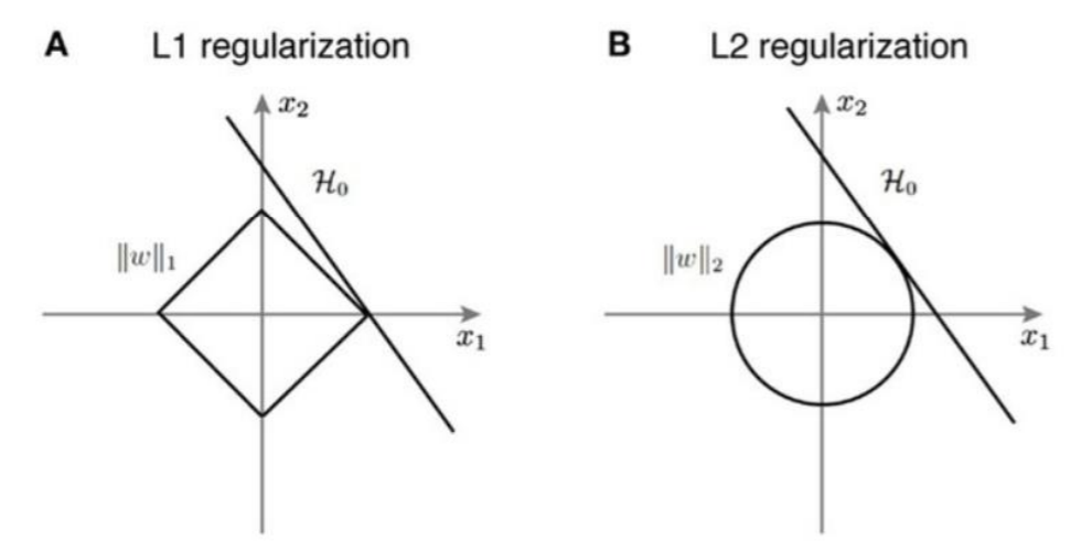
Now let’s understand both methods graphically.
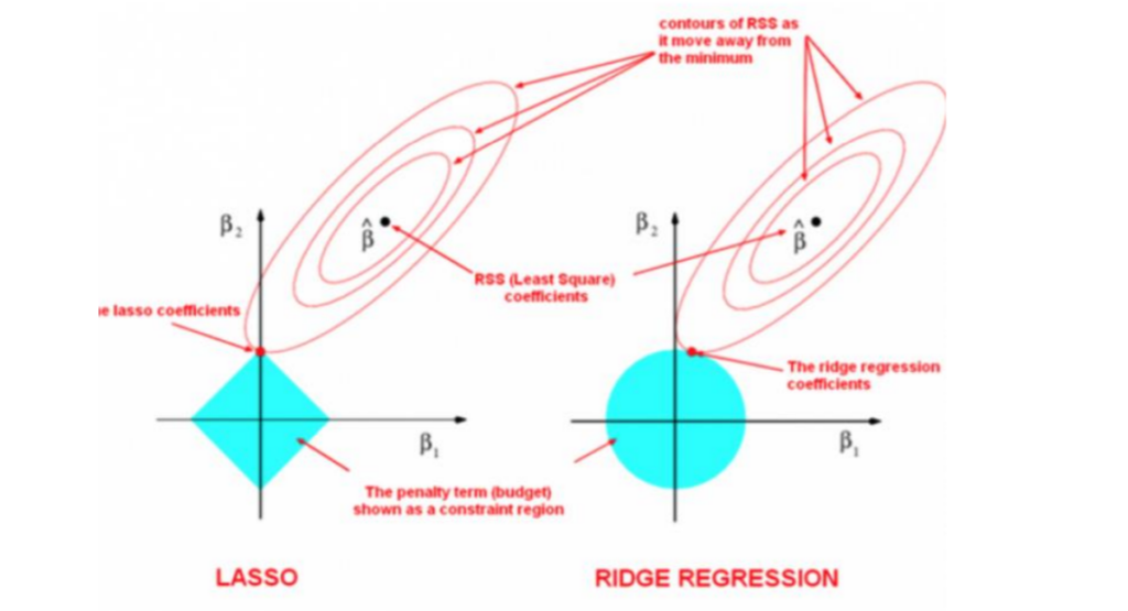
In case of Lasso, the Penalty term is linear equation with each term is the modulus value. Hence, take an example of two coefficient in Lasso Penalty, that will be |β1|+|β2|, if will plot over axis, it will straight line in each quadrant, hence, it will create a diamond shape region, for Ridge Penalty, the term is β1 2+β2 2 , this is equation of circle, hence any point in the circular region will reduce the loss function. Regularization is one of the ways to tradeoff between bias and variance. It reduces the variance while little or no change in bias. Regularization can be easily implemented through Scikit-Learn in Python with few lines of coding.
