In statistics, exploratory data analysis is an approach to analyzing data sets to summarize their main characteristics, often with visual methods. To train a dataset in machine learning, we need to make sure that our data is clean, that is free of missing values and unwanted variables. Cleaning our dataset will result in faster and accurate results. Data exploration is the tool that will come in handy for this purpose.
In this blog, I will discuss all the steps of data exploration and preparation along with the missing value treatment. To explain this more clearly, I’ll be using the ‘Titanic’ dataset from Kaggle.
TABLE OF CONTENT:
I. Steps of Data Exploration and Preparation.
• Variable Identification
• Univariate Analysis
• Bi-variate Analysis
II. Missing value treatment
• Why missing values treatment is required?
• Why data has missing values?
• Methods of treating these missing value.
I. Steps of Data Exploration and Preparation:
Data exploration, cleaning and preparation can take upto 70% of our total project time. In this section, we will learn how to clean and prepare our data for building predictive model.
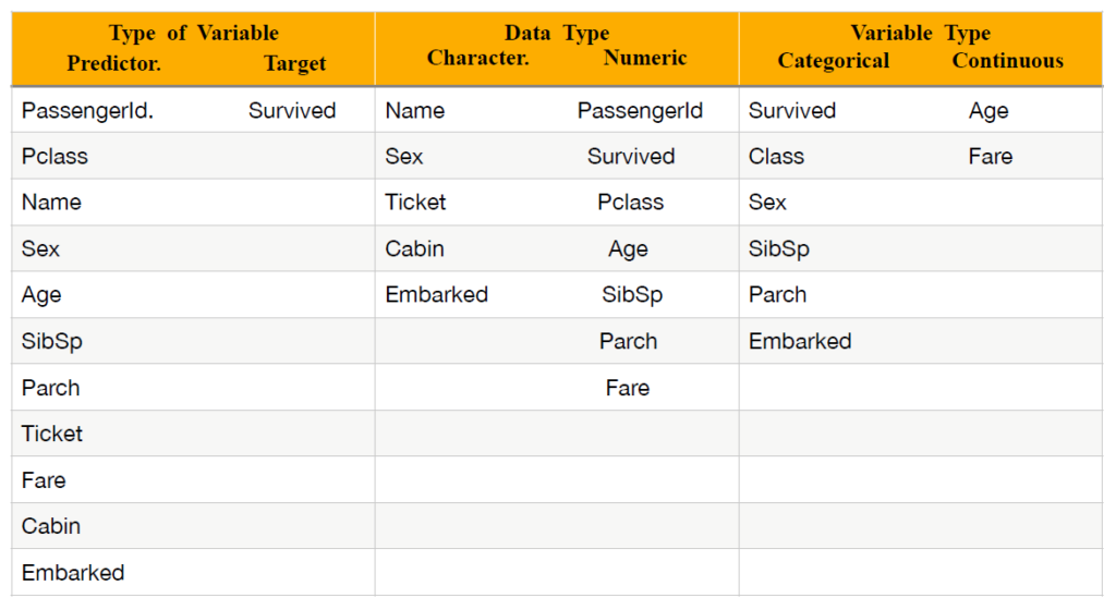
• Variable Identification: We start by identifying our Predictor/Input and Target/Output variable and the category of the variables. In our Titanic dataset model we have to predict the survived passenger. Here we need to identify predictor variables, target variable, data type of variables and category of variables.

Below, the variables have been defined in different category:
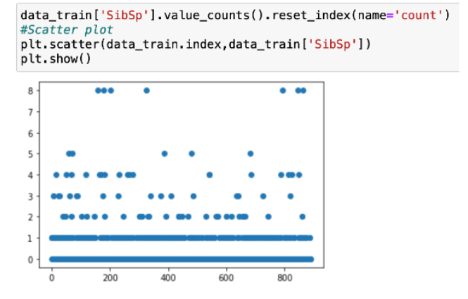
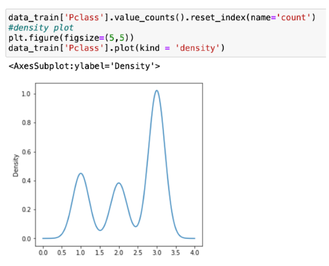
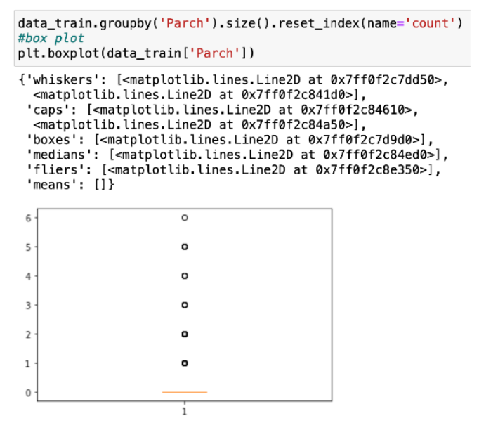
• Univariate Analysis: At this stage, we will explore the variables one by one. This method depends on the variable type i.e. whether the variable is categorical or continuous. We will use different kinds of visualizations like density plots, scatter plots and box plots for better understanding.
- Categorical variable: For categorical variables, we’ll use frequency table to understand distribution of each category. We can also read as percentage of values under each category. We have six categorical variables in our dataset. Here are the visual representation for each one of them.


- Continuous variable: In case of continuous variables, we need to understand the central tendency and spread of the variable. We will use histograms to plot the continuous variables.
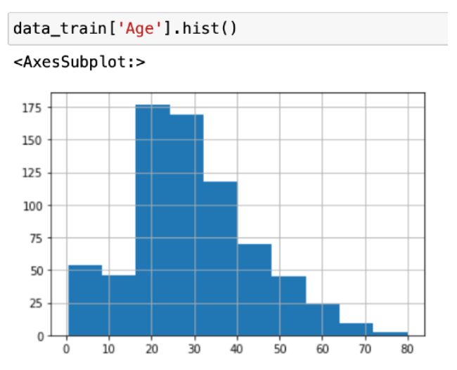
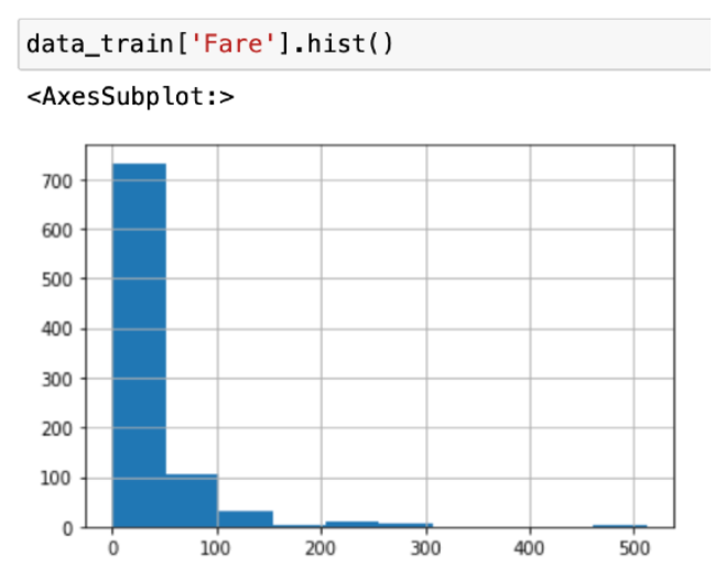
• Bi-variate Analysis: Bi-variate Analysis finds out the relationship between two variables. Here, we look for association and disassociation between variables at a pre-defined significance level. We can perform bi-variate analysis for any combination of categorical and continuous variables. The combination can be Categorical & Categorical, Categorical & Continuous and Continuous & Continuous. Different methods are used to tackle these combinations during analysis process. But all of them can be handled by Correlation. We will use heat map to visualize this.
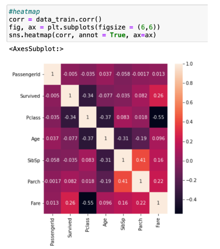
From the heat map we can see that variable survived is highly related with Fare and poorly related with Pclass. So, from this we can say that Fare will play an important part in classification.
II. Missing Value Treatment:
• Why missing values treatment is required?
Missing data in the training data set can reduce the power / fit of a model or can lead to a biased model because we have not analyzed the behavior and relationship with other variables correctly. It can lead to wrong prediction or classification.
• Why data has missing values?
Data Extraction: It is possible that there are problems with extraction process. In such cases, we should double-check for correct data with data guardians. Some hashing procedures can also be used to make sure data extraction is correct. Errors at data extraction stage are typically easy to find and can be corrected easily as well.
Data collection: These errors occur at time of data collection and are harder to correct. They can be categorized in four types:
- Missing completely at random: This is a case when the probability of missing variable is same for all observations. For example: respondents of data collection process decide
that they will declare their earning after tossing a fair coin. If an head occurs, respondent declares his / her earnings & vice versa. Here each observation has equal chance of missing value. - Missing at random: This is a case when variable is missing at random and missing ratio varies for different values / level of other input variables. For example: We are collecting data for age and female has higher missing value compare to male.
- Missing that depends on unobserved predictors: This is a case when the missing values are not random and are related to the unobserved input variable. For example: In a medical study, if a particular diagnostic causes discomfort, then there is higher chance of drop out from the study. This missing value is not at random unless we have included “discomfort” as an input variable for all patients.
- Missing depends on the missing value itself: This is case when the probability of missing value is directly correlated with missing value itself. For example: People with higher or lower income are likely to provide non-response to their earning.
• Methods of treating missing values:
- By removing the rows with null values: Simplicity is one of the major advantage of this method, but this method reduces the power of model because it reduces the sample size.
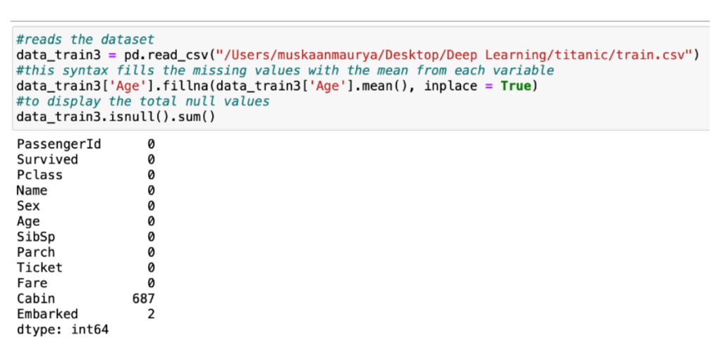
- By imputation (mean): Imputation is a method to fill in the missing values with estimated ones. The objective is to employ known relationships that can be identified in the valid values of the data set to assist in estimating the missing values. Mean imputation is one of the most frequently used methods. It consists of replacing the missing data for a given attribute by the mean or median (quantitative attribute) or mode (qualitative attribute) of all known values of that variable. Evidently, this works only on numeric variables.
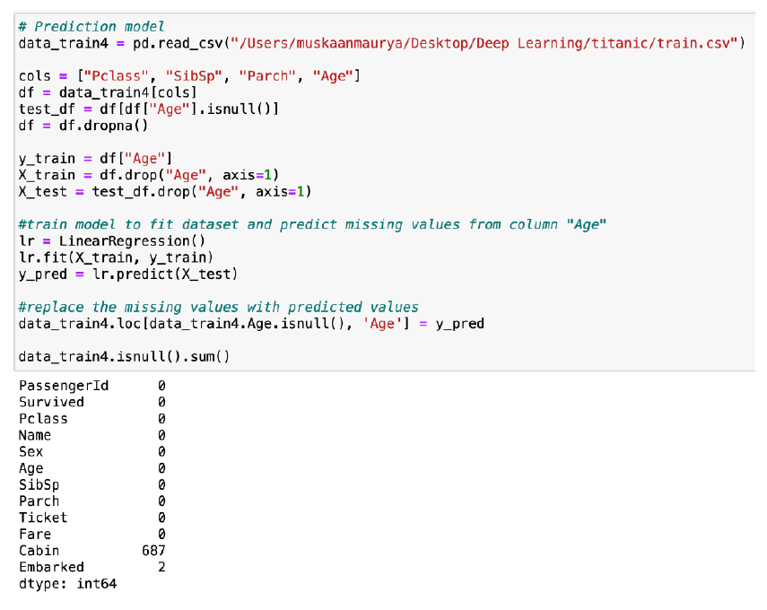
3. By prediction model :
Prediction model is one of the sophisticated method for handling missing data. Here, we create a predictive model to estimate values that will substitute the missing data. In this case, we divide our data set into two sets: One set with no missing values for the
variable and another one with missing values. First data set become training data set of the model while second data set with missing values is test data set and variable with missing values is treated as target variable. Next, we create a model to predict target variable based on other attributes of the training data set and populate missing values of
test data set.We can use regression, ANOVA, Logistic regression and various modelling technique to perform this. There are 2 drawbacks for this approach:
- The model estimated values are usually more well-behaved than
the true values - If there are no relationships with attributes in the data set and the
attribute with missing values, then the model will not be precise
for estimating missing values.
4. By KNN imputation: In method of imputation, the missing values of an attribute are imputed using the given number of attributes that are most similar to the attribute whose values are missing. The similarity of two attributes is determined using a distance function. It is also known to have certain advantage & disadvantages.
Advantages:
▪ k-nearest neighbour can predict both qualitative & quantitative attributes
▪ Creation of predictive model for each attribute with missing data is not required
▪ Attributes with multiple missing values can be easily treated
▪ Correlation structure
Disadvantages:
▪ KNN algorithm is very time-consuming in analyzing
large database. It searches through all the dataset
looking for the most similar instances.
▪ Choice of k-value is very critical. Higher value of k would include attributes which are significantly different from what we need whereas lower value of k implies missing out of significant attributes
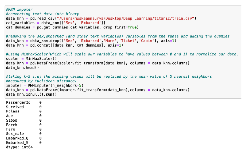
Now, we have successfully removed all the missing values. EDA is followed by training of the dataset to get the desired result.
Conclusion
As mentioned in the beginning, quality and efforts invested in data exploration
differentiates a good model from a bad model. In this blog, I have discussed the crucial steps needed to perform EDA, in details.
References:
• towardsdatascience.com
• analyticalvidhya.com
• “Titanic” dataset : https://www.kaggle.com/c/titanic/data
