Convolution Neural Network

Introduction:

In deep learning, a convolutional neural network (CNN, or ConvNet) is a class of deep neural networks, most commonly applied to analyzing visual imagery.

Convolutional Neural Networks are very similar to ordinary Neural Networks they are made up of neurons that have learnable weights and biases. Each neuron receives some inputs, performs a dot product and optionally follows it with a non-linearity. The whole network still expresses a single differentiable score function: from the raw image pixels on one end to class scores at the other. And they still have a loss function (e.g. SVM/Softmax) on the last (fully-connected) layer and all the tips/tricks we developed for learning regular Neural Networks still apply.

So what does change? ConvNet architectures make the explicit assumption that the inputs are images, which allows us to encode certain properties into the architecture. These then make the forward function more efficient to implement and vastly reduce the amount of parameters in the network.

We can find that they have applications in image and video recognition, recommender   systems,image classification, medical image analysis, natural language processing and financial time series.

Before deep diving into neural networks, understanding the algorithmns, the first question which should come in our mind is how our computer understand an image? We will start learning by answering this question!

How a computer reads an image?

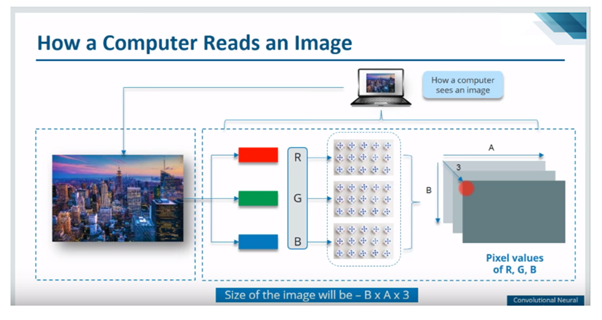
As you can see in the image below, there are three channels Red, Green & Blue, which is popularly known as R, G & B. They have their respective pixel values. So If we will say size of image is – B x A x 3. It means there are “B” rows, “A” columns and 3 channels e.g if the image size is 28 x 28 x 3, it means 28 rows, 28 columns and 3 channels. It is applicable for any coloured image. This is how our computer see the images. While if image is Black & White image, we have only 2 channels.

Why not we use fully connected network for CNN?

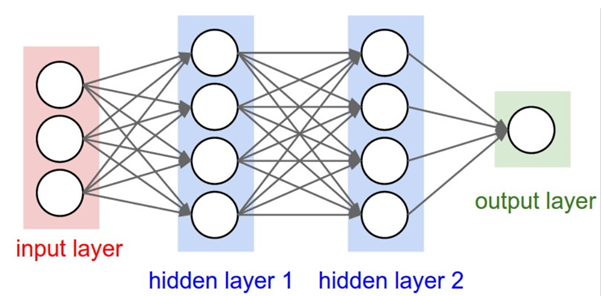
From the image below, consider a 28 x 28 x 3 pixel image and feed it into fully connected network, then the total number of weights in the first hidden layer will be 2352. But in real-time images are bigger, so it will be bigger than 200 x 200 x 3, and the numbers of weight in the first hidden layer itself will be 120,000. So, we have to deal with such huge amount of parameters and we will require more number of neurons and it will lead to overfitting. That is why we don’t use fully connected networks for image classification.

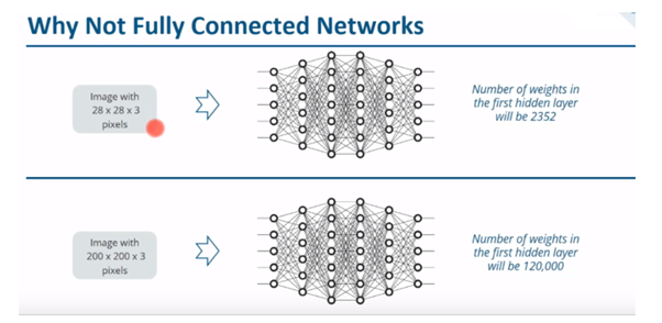
Regular Neural Nets don’t scale well to full images. In CIFAR-10, images are only of size 32x32x3 (32 wide, 32 high, 3 colour channels), so a single fully-connected neuron in a first hidden layer of a regular Neural Network would have 32323 = 3072 weights. This amount still seems manageable, but clearly this fully-connected structure does not scale to larger images. For example, an image of more respectable size, e.g. 200x200x3, would lead to neurons that have 2002003 = 120,000 weights. Moreover, we would almost certainly want to have several such neurons, so the parameters would add up quickly! Clearly, this full connectivity is wasteful and the huge number of parameters would quickly lead to overfitting.

Why we need Convolutional Neural Networks?

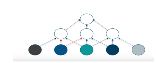
In case of a convolutional neural network, a neuron in a layer will only be connected to a small region of the layer of the layer before it, instead of all of neurons in a fully-connected manner, because we need to handle less amount of weight and we need less number of neurons as well.

Below Image clearly explains how each neurons are fully connected.

Intuition behind Convolutional Neural Networks

Convolutional Neural Network (CNN, or ConvNet) is a type of feed- forward artificial neural network in which the connectivity between its neurons is inspired by the organization of the animal visual cortex.

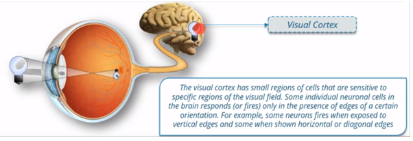
Visual cortex is nothing but a small region in our brain which is present in form of bulb in below diagram. There was a experiment conducted and people found that Visual cortex is small region of cells that are sensitive to specific region of visual field. For example, some neurons in the visual cortex fires when expose to vertical edges and some fires when exposes to horizontal edges and some will fires to diagonal edges and that is motivation behind convolution neural network.

3D volumes of neurons. Convolutional Neural Networks take advantage of the fact that the input consists of images and they constrain the architecture in a more sensible way. In particular, unlike a regular Neural Network, the layers of a ConvNet have neurons arranged in 3 dimensions: width, height, depth. (Note that the word depth here refers to the third dimension of an activation volume, not to the depth of a full Neural Network, which can refer to the total number of layers in a network.)

For example, the input images in CIFAR-10 are an input volume of activations, and the volume has dimensions 32x32x3 (width, height, depth respectively). As we will soon see, the neurons in a layer will only be connected to a small region of the layer before it, instead of all of the neurons in a fully-connected manner.

Moreover, the final output layer would for CIFAR-10 have dimensions 1x1x10, because by the end of the ConvNet architecture we will reduce the full image into a single vector of class scores, arranged along the depth dimension. Here is a visualization:

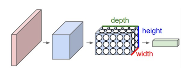
A ConvNet arranges its neurons in three dimensions (width, height, depth), as visualized in one of the layers. Every layer of a ConvNet transforms the 3D input volume to a 3D output volume of neuron activations. In this example, the red input layer holds the image, so its width and height would be the dimensions of the image, and the depth would be 3 (Red, Green, Blue channels).

A ConvNet is made up of Layers. Every Layer has a simple API: It transforms an input 3D volume to an output 3D volume with some differentiable function that may or may not have parameters.

How convolutional neural network works?

Convolutional Neural Networks have following layers :

A simple ConvNet is a sequence of layers, and every layer of a ConvNet transforms one volume of activations to another through a differentiable function. We use five main types of layers to build ConvNet architectures: Input Layer,Convolutional Layer, Relu Layer,Pooling Layer, and Fully-Connected Layer (exactly as seen in the image below). We will stack these layers to form a full ConvNet architecture.

1. The input layer
2. The convolution layer
3. The ReLu layer
4. The Pooling layer
5. The fully connected layer

Why 3D layers?

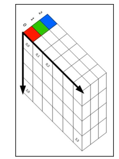
3D layers allow us to use convolutions to learn the image features. This helps the network decrease its training time as there will be less weight in the deep network. The three dimensions of an image are as follows:

• Height
• Width
• Depth (RGB)

The 3D layers of an image can be seen in the following screenshot:

Let’s start with the Convolution Layer.

The convolution layer is the most important part of a CNN as it is the layer that learns the image features. Before we dive deep into convolutions, we must know about image features.

Image features are the part of the image that we are most interested in. Some examples of image features are as follows:

• Edges
• Colors
• Patterns/shapes

Before CNNs, the extraction of features from an image was a tedious process—the feature engineering done for one set of images would not be appropriate for another set of images.

Let’s try to understand what convolution is. In simple terms, convolution is a mathematical term to describe the process of combining two functions to produce a third function. The third function, or the output, is called the feature map. Convolution is the action of using a kernel or filter applied to an input image, and the output is the feature map. The convolution feature is executed by sliding a kernel over the input image. Generally, the convolution-sliding process is done with a simple matrix multiplication or dot product.

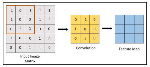
Now, we will see an example of how convolution works:

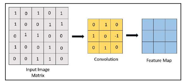
In the following steps, we will learn to create a feature map using convolution:

1.The first step is to slide over the image matrix, as shown in the image below:

2. The next step is to multiply the convolution by the input image matrix:

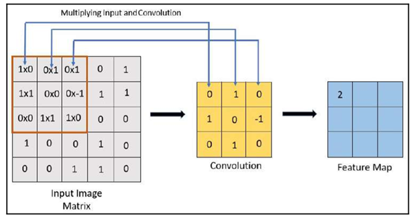
In the above image, we can see how the feature map is created after the convolution kernel is applied:

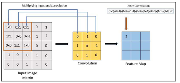
3. Now, we will slide the kernel to get the next feature map output

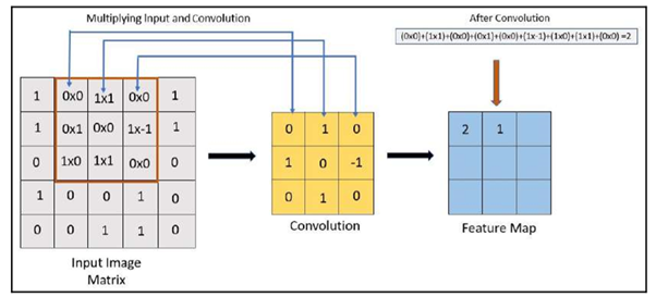
In the preceding example, the 3 x 3 kernel slides 9 times.

We will get the 9 values as the feature map result. Here are a few important points on the effect of kernels:

• The kernel produces scalar outputs.
• The result of the feature map depends on the value of the kernels.
• Convolving with different kernels produces interesting feature maps that can be used to detect different features.
• After compressing the feature in the form of a feature map, the convolution keeps the spatial relationship by retaining the compressed information of the image.

In CNNs, we can use many filters.

For example, if we have 12 filters in a CNN, and we apply 12 filters with a size of 3 x 3 x 3 to our input image with a size of 28 x 28 x 3, we will produce 12 feature maps, also known as activation maps. These outputs are stacked together and treated as another 3D matrix, but in our example, the size of the output will be 28 x 28 x 12. This 3D output will then be inputted to the next layer of the CNN.

Depth, stride, and padding

Depth, stride, and padding are the hyperparameters used to tweak the size of the convolutional filters. In the previous section, Understanding the convolution layer, we applied 3 x 3 filters or kernels for the convolution of a CNN.

But the question is, does the filter have to be 3 x 3? How many filters do we need? Are we going to shift over pixel by pixel? We can have filters of greater size than 3 x 3. It is possible to do this by tweaking the following parameters. You can also tweak these parameters to control the size of the feature maps:

• Kernel size (K x K)
• Depth
• Stride
• Padding

Depth

Depth tells us the number of filters used. It does not relate to the image depth, nor to the number of hidden layers in the CNN. Each filter or kernel learns different feature maps that are activated in the presence of different image features, such as edges, patterns, and colors.

Stride

Stride basically refers to the step size we take when we slide the kernel across the input image.

An example of a stride of 1 is shown in the following image:

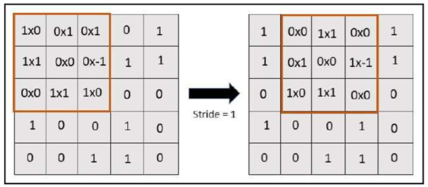
In a stride of 1, the value of the feature map is 9. Similarly, a stride of 2 looks as follows:

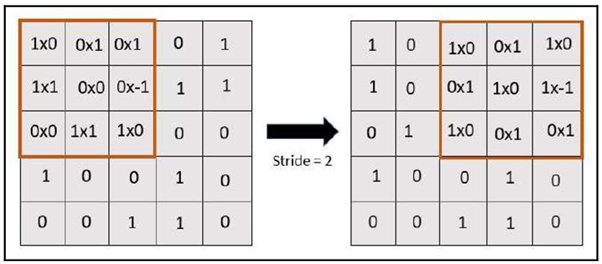
When we have a stride of 2, the value of the feature map will be 4, which is equivalent to 2 x 2.

Stride is important because of the following points:

• The stride controls the size of the convolution layer output.
• Using larger strides produces less overlap in kernels.
• Stride is one of the methods to control the spatial input size—that is, passing information to other input layers without losing it.

Zero-padding

Zero-padding is a very simple concept that we apply to the border of our input. With a stride of 1, the output of the feature map will be a 3 x 3 matrix. We can see that after applying a stride of 1, we end up with a tiny output. This output will be the input for the next layer. In this way, there are high chances of losing information.

So, we add a border of zeros around the input, as shown in the following image:

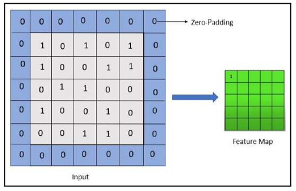
Adding zeros around the border is equivalent to adding a black border around an image.

We can also set the padding to 2 if required. Now, we will calculate the output of the convolution mathematically.

We have the following parameters:

• Kernal/filter size, K
• Depth,D
• Stride,S
• Zero-padding, P
• Input image size, I

To ensure that the filters cover the full input image symmetrically, we’ll use the following equation to do the sanity check; it is valid if the result of the equation is an integer:

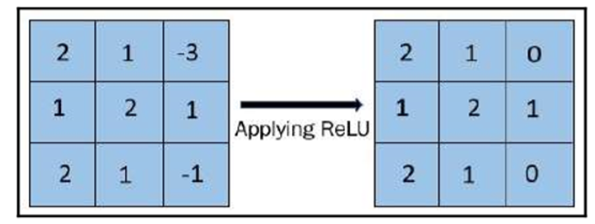
Let’s have a look  about the activation function known as Rectified Linear Unit (ReLU).

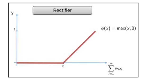
An example of ReLU introducing non-linearity in the feature map’s output can be seen in the following image:

Fully connected layers

Having fully connected layers simply means that all the nodes in one layer are connected to the outputs of the next layers. The output of the fully connected layer is a class of probabilities, where each class is assigned a probability. All probabilities must sum up to 1. The activation function used at the output of the layer is called the softmax function.

The softmax function

The activation function used to produce the probabilities per class is called the softmax function. It turns the output of the fully connected layer, or the last layer, into probabilities. The sum of the probabilities of the classes is 1 – Panda = 0.04, Cat = 0.91, and Dog = 0.05, which totals 1. We can see the values of the softmax function in the following image: