Case Study: Reducing Commercial Aviation Fatalities

Overview
Business Problem
Dataset Analysis
Mapping the Real Problem into ML problem
Performance Metric
Exploratory Data Analysis
Feature Engineering
Data preprocessing
Modeling
Future improvements
Results
References

Overview

Source: https://www.kaggle.com/c/reducing-commercial-aviation-fatalities

This was a competition conducted by Kaggle where we needed to build a model to detect troubling events from aircrew’s physiological data.

Aviation fatality means the death of one or more persons inside or outside of an aircraft, spacecraft, or any other aerospace vehicle that occurs during a flight operation or any other operation involving that vehicle. These fatalities are directly associated with the operation of the aircraft and are called aviation accidents.

The most frequent causes for these aviation accidents include:

Pilot error
Mechanical failure
Design defect
Air traffic failure
Defective runways

In this competition, the main focus is on the first cause i.e, aviation accidents caused by pilot error, and solutions to avoid them.

Business Problem

A large part of the training given to the pilot involves the physiological aspects which are required while flying an airplane. This is important because one of the important abilities required for pilots is to multitask, the ability to concentrate, and the ability to pay attention to all these tasks. All of these may help to reduce pilot induced flight fatalities.

Most of the flight fatalities or flight accidents due to pilot error are due to the loss of airplane state awareness. Airplane state awareness (ASA) is a pilot performance attribute wherein the pilot should be able to realize and respond quickly to any change of state of the airplane. Loss of airplane state awareness may lead to many dangerous situations and may result in loss of airplane control wherein an extreme deviation from the intended flight path may occur. Loss of ASA is mainly due to loss of attention on the part of pilots who may be distracted, sleepy, or in other dangerous cognitive states. Due to the stressful environment, while flying, the possibility of the loss of awareness is common.

In this competition, we are provided with real physiological data from pilots who were subjected to various distracting events. The pilots experienced distractions and resulted in one of the following three cognitive states:

Channelized Attention (CA): This occurs when the pilot is focusing only on one task without giving any attention to other tasks.
Diverted Attention (DA): The state of having one’s attention diverted by actions or thought processes associated with a decision. This is induced by having the subjects perform a display monitoring task.
Startle/Surprise (SS): This is the response to a sudden unexpected stimulus. In aviation, this can be defined as an uncontrollable automatic reflex or reaction caused due to exposure to a sudden intense event that violated a pilot’s expectations.

The aim is to build a model that can estimate the state of mind of the pilot in real-time using the physiological data given. When the pilot enters into any one of the above mentioned dangerous cognitive states, he/she should be alerted, thereby preventing any possible accident.

Dataset Analysis

Three CSV files are provided for this competition. The first one is train.csv in which all the data is to be used for training. Test.csv is provided to test the model. Sample_submission.csv is provided to submit the final output in the CSV format.

Now, let’s analyze each attribute in the dataset.

The training data consist of three experiments: CA, DA, and SS. The output is one of the four labels: Baseline(no event), CA, DA, or SS. For example, if the experiment is CA, the output is either CA or Baseline(no event). The test data is taken from a full flight simulator. Here the experiment is called LOFT or Line Oriented Flight Training where the training of the pilot is carried out in a flight simulator, which artificially creates the environment of a real flight. In the test data, the experiment is given as LOFT and the output can be one of the four states at a given time. To predict the state of a pilot, physiological data are required. We have data from four sensors — EEG, ECG, Respiration, Galvanic skin response. Let’s analyze each attribute of the dataset.

Id: Unique identifier for crew+time combination. A pilot with a particular time into the experiment is represented using an id. So for each id, we need to predict the state
Crew: Unique id for a pair or pilot
Experiment: For training, it will be either CA or DA or SS. For testing, it will be LOFT
Time: Seconds into the experiment
Seat: Seat of the pilot- 0 means left, 1 means right

EEG (Electroencephalogram) — This is the summation of all activities on the surface of the brain. Data from 20 electrodes are given to us. Each electrode lead is placed near a particular part of the brain ( prefrontal(fp), temporal(t), frontal(f), parietal(p), occipital(o), central(c) ). The odd numbers in the representation indicate that the electrode is placed on the left side of the brain, even numbers indicate the right side, and z indicate the middle region.

The below figure gives an idea about the position of each electrode.

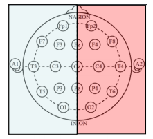
Figure 1: Position of electrodes in the scalp

Eeg_f7: Data from the electrode near the prefrontal portion — left side
Eeg_f8: Data from the electrode near the frontal area — right side
Eeg_t4: Data from the electrode near the temporal area — right side
Eeg_t6: Data from the electrode near the temporal area — right side
Eeg_t5: Data from the electrode near the temporal area — left side
Eeg_t3: Data from the electrode near the temporal area — left side
Eeg_fp2: Data from the electrode near the prefrontal area — right side
Eeg_o1: Data from the electrode near the occipital area — left side
Eeg_p3: Data from the electrode near the parietal area — left side
Eeg_pz: Data from the electrode near the parietal area — middle region
Eeg_f3: Data from the electrode near the frontal area — left side
Eeg_fz: Data from the electrode near the frontal area — middle region
Eeg_f4: Data from the electrode near the frontal area — right side
Eeg_c4: Data from the electrode near the central area — right side
Eeg_p4: Data from the electrode near the parietal area — right side
Eeg_poz: Data from the electrode near the parietal-occipital junction — Middle region
Eeg_c3: Data from the electrode near the central area — left side
Eeg_cz: Data from the electrode near the central area — middle region
Eeg_o2: Data from the electrode near the occipital area — right side

Ecg: Three-point electrocardiogram (ECG) signal — It measures the electrical activity of the heart (sensor output is in microvolts)
R: Respiration sensor — It measures the rise and fall of the chest (Sensor output is in microvolts)
Gsr: Galvanic skin response — The measure of electrodermal activity (Sensor output is in microvolts)
Event: The output which is to be predicted — The state of the pilot at a given time. It will be either baseline (A no event) or SS(B) or CA(C)or DA(D)

Mapping the Real Problem into ML problem

This is a multiclass classification problem wherein, for each id (for a particular crew at a particular time), we need to predict the state of the pilot as belonging to one of the four given classes. Given all the attributes, we need to predict the probability of occurrence of each event.

Performance Metric

The problem we are handling is a multiclass classification problem where the number of classes is 4

The evaluation matrix used in this competition is multiclass log loss

where N is the total number of data points, M is the number of classes.

yij is 1 if the data point i is predicted to be of class j, and is 0 otherwise.

pij is the probability of datapoint i belonging to class j

We can also use precision and recall matrices for evaluating the performance where we can check how well we were able to predict and recall each of the states. i.e, for each of the “dangerous state” classes, we should be able to correctly predict maximum data points in these classes and we should not misclassify it as a normal state.

Exploratory Data Analysis(EDA)

Analyze the events

First and foremost, let’s analyze the frequency of occurrence of each of the events. We can use the count plot(paste link) for this.

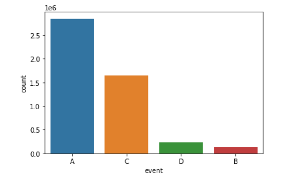
Figure 2: The frequency of events

Here A indicates Baseline(no event), B indicates Startle/Surprise, C indicates CA, and D indicates DA. From this plot, it is clear that the data is imbalanced. Or we can say, the frequency of occurrence of each event is different. Let’s go one level deeper and analyze each event.

Let’s consider each of the experiments separately and consider a randomly selected crew and analyze the frequency of each event.

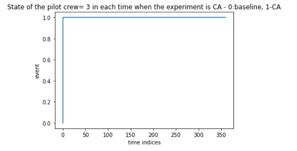
Figure 3: Analyzing the frequency of CA event

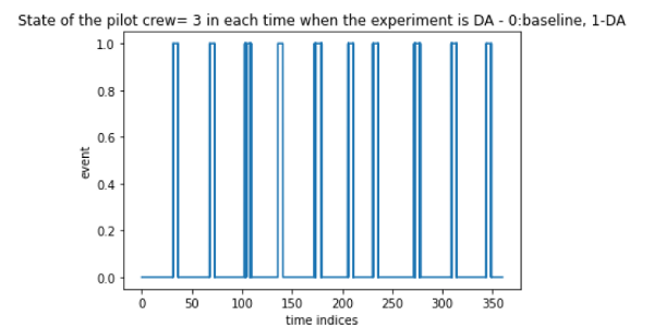
Figure 4: Analyzing the frequency of DA event

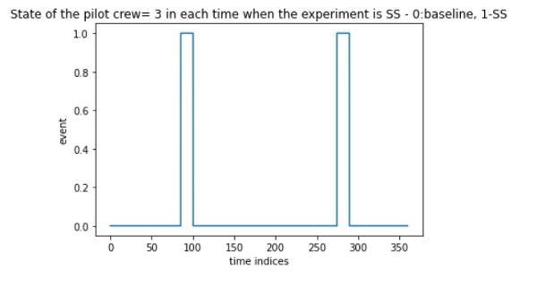
Figure 5: Analyzing the frequency of SS event

So from these figures, we can say that all the experiments are conducted for the same interval, yet the frequency of occurrence of SS is very low. This frequency imbalance is possible in the test dataset also, so we keep this imbalance for the time being and check the performance without balancing the dataset.

Univariate analysis for each feature

Here we use box plots for analyzing the effect of each feature in predicting the event.

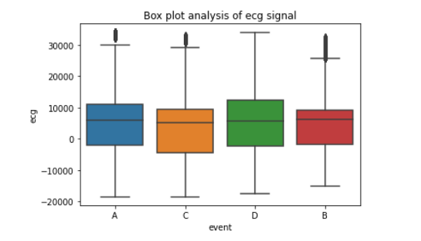
Figure 6: Box plot of ECG data

From the above figure, it can be seen that the ECG data has some outliers. But we cannot simply remove them because these extreme values might be useful in predicting the event. When the value of ECG is high (more than 10000 microvolts), the pilot is more likely to enter into the DA state. Similarly, when the value is too negative, the pilot is likely to be in the CA state. It is also observed that ECG alone cannot simply predict the events. But it has some role in prediction

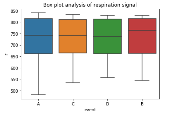
Figure 7: Box plot of respiration sensor output data

Similar to ECG data this data also has some outliers. But we cannot simply remove them because these extreme values might be useful in predicting the event. The respiration signal should have some effect in predicting the event, But from the above box plot, we can see that this sensor output is not at all separating the events. This might be because of the presence of noise in the data.

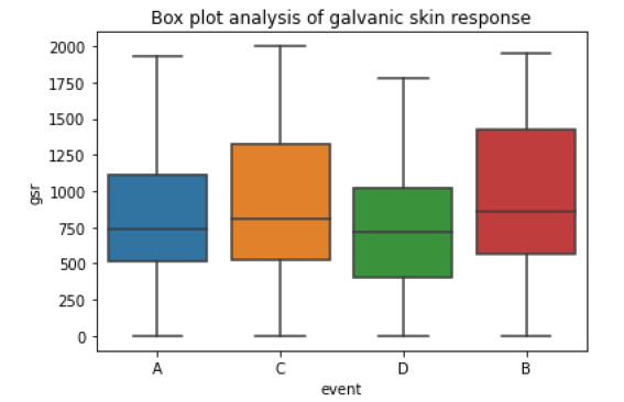
Figure 8: box plot of GSR sensor output

From the box plot of GSR, we can say that GSR plays some role in predicting the output. This GSR data is separating the events to some extent.

Now the next step is to check for noise in the data. The biological sensors are easily affected by noise and since the data is obtained from the physiological data of real people, the output from these sensors will be rich in noises. Let’s check noise in ECG and R data. This data is analyzed for the experiment and for a particular crew.

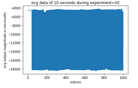
Figure 9: ECG output data for 10 seconds

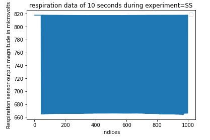
Figure 10: Respiration sensor data for 10 seconds

These data are clearly rich in noise and hence we need to remove this high-frequency noise. For that purpose, we use a low pass Butterworth filter.

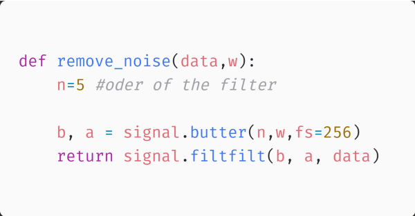
For filtering the ECG signal, the cutoff frequency(w) was selected as 100 and for filtering the respiration signal, the value of w was taken as 0.7. The filtered ECG and r signal is shown below.

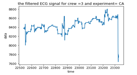
Figure 11: Filtered ECG data

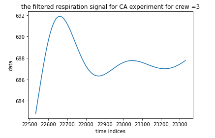
Figure 12: Filtered respiration data

The filtered data are much cleaner and meaningful than the original data. So we replace the ECG and r data with the corresponding filtered signals.

Feature Engineering

Now let’s try to derive some additional features from the existing ones.

Heart Beat information from ECG

What if we could get the heartbeat from the ECG signal?

ECG is the graph showing the electrical activity of the heart vs time. The output from ECG is in microvolts. Now, apart from this voltage, we can get the cardiac output or heart rate or the number of heartbeats per min using this data. Python provides a powerful tool called Biosppy which can do biosignal processing.

As you can see it is very simple to obtain all the necessary information from ECG using this module

Respiration rate from r signal

It is the rise and fall of the chest. It represents the muscular activity of the abdomen and diaphragm. So when a person is stressed or shocked, the rate of respiration will be high. How can we obtain the respiration rate from the respiration sensor output?

As in the case of ECG, here also we can use Biosppy to derive the respiration rate from the r signal.

So we got the heart rate and respiration rate from the Biosppy module at particular time stamps. In order to get the data corresponding to all the timestamps in our dataset, we can do the interpolation technique.

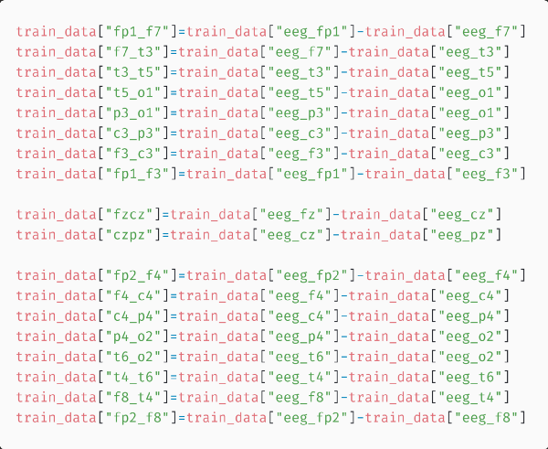
The potential difference between the EEG electrodes

In this competition, we are given the voltage from 20 electrodes placed in different parts of the brain as shown in figure1. For clinical purposes, the potential difference between the electrodes is considered a more important feature. This potential difference will give us an idea about the electrical field in that brain region and the state of that region.

Now while deriving the potential difference, we can use any of the electrode combinations as shown in figure:

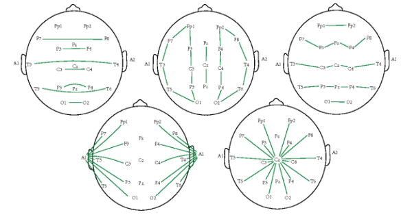
Figure 13: The various montages for finding the potential difference between the EEG electrodes

Here I used the second combination because it is mostly used in clinics

Frequency band information from the EEG signals

A typical adult human EEG signal is about 10 µV to 100 µV in amplitude when measured from the scalp. The wave associated with each electrode is a combination of multiple waves with different amplitudes and frequencies as shown in the figure.

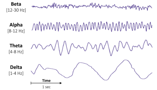
Figure 14: The various frequency components in an EEG electrode output

The significance of these frequency bands of ECG in determining the mental state of a person is as described below:

Delta(1 to 4Hz): This rhythm is prominently observed in deep sleep. A very high amplitude indicates brain injuries, learning problems, inability to think, etc. A very low amplitude indicates the inability to rejuvenate the body, inability to revitalize the brain, poor sleep, etc.
Theta (4 to 8Hz): This rhythm is usually observed during drowsiness as well as in the early stages of sleep. This can also arise due to heightened emotional states. A very high amplitude indicates ADHD, depression, hyperactivity, inattentiveness, etc. A very low amplitude indicates anxiety, poor emotional awareness, stress, etc.
Alpha (8 to 12 Hz): This rhythm is usually observed in the EEG when the person is awake. The amplitude of these waves may vary across different individuals and different mental states of an individual. A very high amplitude indicates daydreaming, inability to focus, etc. A very low amplitude indicates anxiety, high stress, insomnia, OCD, etc.
Beta (12 to 30 Hz): This is the most commonly and frequently observed rhythm in adults and children. The amplitude of a beta wave is usually between 10 to 20 microvolts. A very high amplitude indicates anxiety, high arousal, inability to relax, stress, etc. A very low value indicates ADHD, daydreaming, depression, poor cognition, etc.
Gamma (>30 Hz): High value indicates Anxiety, high arousal, stress, etc. A very low value indicates ADHD, depression, learning disabilities, etc.

Here we can use theBiosppy for deriving all the frequency band information.

Finally, we remove all the redundant features like the experiment, seat, noisy ECG, and noisy r. We also ignore the gamma and beta features, because the contribution of these features was very low when we observed the correlation matrix. These features increase the dimensionality of the data without contributing much to the prediction.

Feature Importance

Now let’s see the importance of each of these features in predicting the output. I have used the Random Forest Classifier for obtaining the importance of the features.

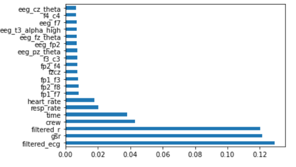
Figure 15: The feature importance of top 20 features computed using Random Forest

Here, I have analyzed the top 20 important features. This mostly consists of derived features. So we can conclude that the engineered features are important.

Data preprocessing

Here I have used StandardScaler for standardizing the data. Standardization of a dataset is a common requirement for many machine learning estimators. The models might behave badly if the individual features do not more or less look like standard normally distributed data.

Modeling

Considering the number of features available, tree-based models are expected to perform better. The best model was LightGBM. The best parameters for the model obtained using proper hyperparameter tuning are:

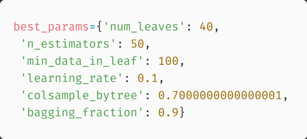
The training data was split into train and cross-validation data. After all the featurization and preprocessing, the data is passed into the model for training.

Results

The multi-class log loss obtained for the train and cross-validation data is shown below.

The test loss is obtained after submitting the results for test data. This is shown below

You can find my complete solution in my Github Repository and if you have any suggestions, please contact me via Linkedin

Future Improvements

Noise removal of EEG data can be done for obtaining a more clean EEG data
From the ECG data, the information about R peak intervals can be obtained

Table of Contents