Table of Contents
- Overview
- Prerequisites
- Business Problem
- Data Analysis
- ML Formulation
- Performance Metric
- Data preparation
- Modeling
- Comparison of models
- Model Deployment
- Future Works
- Profile
- References
1. Overview
Image captioning is one of the most important and challenging tasks in deep learning. It is the process of generation of a textual description for an image. For example, consider the below images.
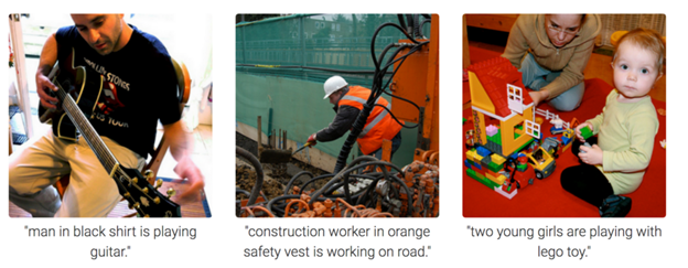
From these images, we humans can come up with a caption or description. But what if the computers can understand the content of the image and generate these captions automatically? This area is called image captioning, and recently the deep learning models have achieved the state of the art performance in this field. The model understands the contents of the image and generates the corresponding textual description. The image captioning process, therefore, can be thought of as a combination of two types of models-
- A model for understanding the contents of the image. Given an image, we need to understand the shapes, edges, colors, etc of the images to get an overall idea about what the image implies. So we need a model that can extract these features and can draw useful insights from the same.
- The second model is for understanding the text. For generating the captions for the image, a model should be able to translate the image features into natural language.
The applications of image captioning include Google Image search, medical report generation, etc.
2. Prerequisites
To understand the blog better, it is better to have some familiarity with topics like Neural networks, CNNs, RNNs, Transfer Learning, Python programming, and Keras library.
3. Business Problem
In this case study, we consider the medical application of image captioning. This case study aims to generate medical reports from a set of chest x-ray images using machine learning algorithms.
An x-ray(radiograph) is a noninvasive medical test that helps physicians diagnose and treat medical conditions. Imaging with x-rays involves exposing a part of the body to a small dose of ionizing radiation to produce pictures of the inside of the body. The chest x-ray is the most commonly performed diagnostic x-ray examination. A chest x-ray produces images of the heart, lungs, airways, blood vessels, and the bones of the spine and chest. Often it is the duty of a radiologist to conclude these x-rays so that to give appropriate treatment to the patients. It is often time-consuming and tedious to get detailed medical reports from these x-rays. In high population countries, a radiologist may come across 100s of x-ray images. So if a properly learned machine learning model can automatically generate these medical reports, considerable work and time can be saved. However, the medical report generated from the model should be confirmed by a radiologist in the final stage.
In this case study, we are using the data given by the Indiana University hospital network. Here a set of chest x-rays and corresponding medical reports are provided. Given an x-ray image, we need to generate the medical report of that x-ray.
4. Data Analysis
The data for this problem is provided by the Indiana University hospital network. The data contains two parts.
- X-rays: http://academictorrents.com/details/5a3a439df24931f410fac269b87b050203d9467d
- Reports: https://academictorrents.com/details/66450ba52ba3f83fbf82ef9c91f2bde0e845aba9
The X-rays contain a set of chest x-ray images for some people. For example,
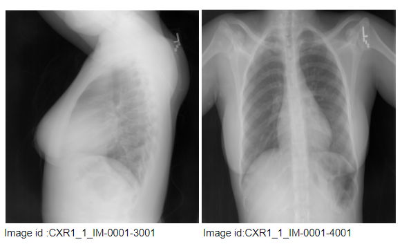
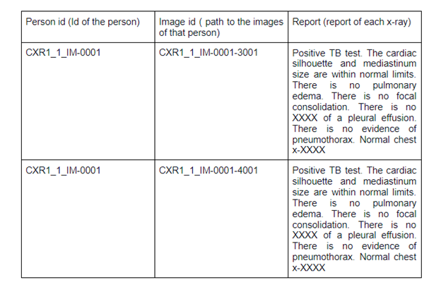
The above figure shows the chest x-ray of a single person. The image id of these images is at the bottom of the images. Here “CXR1_1_1M-001” indicates the id of the patient. The first image is the side view, and the second image is the front view. The image id of these images is shown at the bottom of the images. So there may be one more x-ray image associated with a unique person- report combination.
The reports contain the medical report of an x-ray. Consider the below images of a report
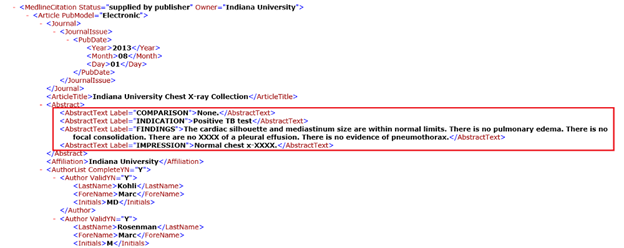
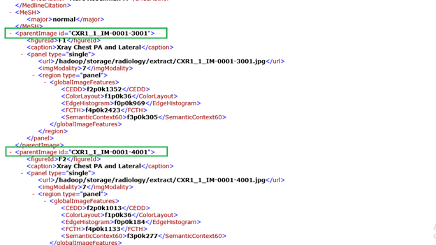
In figure 2(a), the text marked in the red box is what we need to generate as the report of an x-ray. In the impression section, the radiologist provides a diagnosis. The findings section lists the radiology observations regarding each area of the body examined in the imaging study. In figure 2(b), text marked inside the green box indicates the parent image id. Here, the above report is the medical report for the two chest x-rays shown above. Here this report is associated with two images.
A sample dataset will look like:
5. ML Formulation
This problem involves two stages- feature extraction from the images(x-rays) and translates these features into reports. For extracting the image features, we need a convolutional neural network. Usually, pre-trained CNN models are used to get bottleneck features. These features should be given as inputs to some sequence to sequence model for generating reports. These models will give one word as output at a time. These words will be in one hot encoded form. So we need to take the argmax of these one-hot encoded vectors to get the actual words. After t time steps, the model will generate the final report.
6. Performance Metric
For comparing the generated medical reports and actual reports, we can use the BLEU(Bilingual Evaluation Understudy ) score. If the BLEU score is 1, then the generated report and actual report are the same. If the BLEU score is 0, then the generated report and actual report are a perfect mismatch. Since the output from the decoder model is a one-hot encoded vector we can also use categorical cross-entropy as the loss function.
7. Data Preparation
Preparing the text data
The data consists of a set of x-ray images and XML files containing the medical report. As shown in figure 2, this XML has a lot of information like the image id of the x-ray, indication, findings, impression, etc. We will extract the findings and impressions from these files and consider them as reports because they are more useful for the medical report. We also need to extract the image id from these files to get the x-rays corresponding to each report.
If a report does not have findings or image id, we simply drop them
Preprocessing the text data
Let us see some sample reports in our dataset.
Example 1: “Heart size is normal and lungs are clear. Stable 5 mm right midlung perform granuloma.”
Example 2: “No comparison chest x-XXXX. Well-expanded and clear lungs. Mediastinal contour within normal limits..”
We can see that these reports contain special characters, upper case and lower case letters, digits, unwanted spaces, etc. So, we need to clean and preprocess the reports before feeding it into the model. The preprocessed text data is obtained by:
- Convert all letters into lower case
- Words like isn’t, doesn’t, etc are expanded
- Removed all special characters except “.”
- Removed words like “xx”, “xxx”, etc.
- Removed multiple spaces
- Removed words having a length less than or equal to 2
After cleaning the data, the next step is to encode this data into a form for the machine to understand. For that, we need to break the reports into tokens and encode these words into numbers. We use the Keras tokenizer library for this.
It is also observed that the length of each report is different. Before feeding into the model, we need to make all reports to have equal length. This is done using Keras pad sequences.
Preparing the image data
The x-ray corresponding to each report is obtained by extracting the image id from the XML files. It is observed that one report can have multiple x-ray images. We plot the number of x-rays per report to get a better understanding of this.
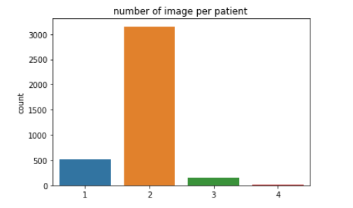
We can see that most of the reports have two images associated with it. It is also observed from the image ids that the images in one report are associated with one patient only. So some patients might have taken multiple x-rays. So, we consider two images of a patient for one report.
The structured data will look like:

Image Featurization
Similar to what we discussed about text encoding, the computer will not be able to understand anything from the image id. To understand the image, we need to convert every image into fixed-sized vectors. This can be done using transfer learning on any pre-trained model. Usually, in all computer vision tasks, CNN models like VGG-16, VGG-19, Inception V3, etc are used.
But transfer learning from these models will not work well here. Why?
The above-pre-trained models are trained on a large dataset which is completely different from the x-ray images. So transfer learning from these models will not provide good results in this case.
So we need a model which is pre-trained on x-ray images. Does such a model exist?
Fortunately yes. Let me introduce you to the CheXNet model. CheXNet is a 121-layer convolutional neural network trained on ChestX-ray14, containing over 100,000 frontal-view X-ray images with 14 diseases. To get the image features using this model, we will remove the final classification layer and extract the output.
You can download the trained weights of CheXNet from here.
The image feature extraction model for CheXNet will look like this.
For easy understanding, let me show you the final layers of the model.
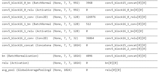
We resize the images into (224,224,3) and pass them to the CheXNet model to get a 1024 dimensional vector. If you remember, we had two images per patient in our data set. So we give both the images into the model to get two image features. Then we concatenate the features to get the final image feature for a patient.
Now that we have converted both text and image data to vectors, we need to split this data into train data and test data. Here we split the data into 80% (train) and 20% (test). Now, let us go to the modeling part.
8. Modeling
From what we have discussed till now, we can say that we need an encoder-decoder architecture for this case study.
- Encoder: This model is used to encode the input into fixed-length vectors.
- Decoder: This model maps the vector representation to a variable-length target sequence.
In our case or in the case of any image captioning problem, the encoder is used to convert the images into vectors. The decoders use Recurrent Neural Networks or LSTMs or GRUs to convert the encoder output into target sentences. The below figure will help to understand this better.

You can understand more about encoder-decoder models for image captioning here.
In this case study, I have used four models of encoder-decoder architecture. Let us try to understand each model.
Model 1: Simple encoder-decoder model
First, let us consider a simple encoder-decoder model.
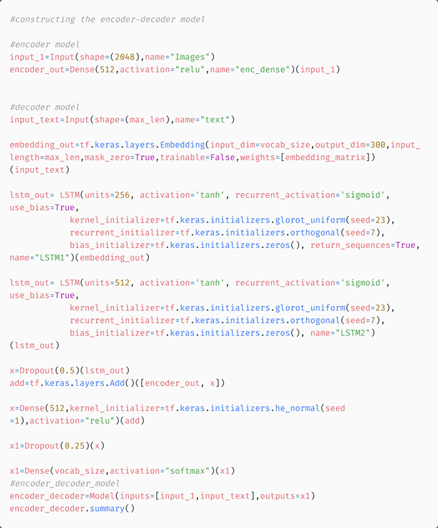
Encoder model: As discussed earlier the encoder model is used to encode the image into fixed-sized vectors. In this case study, we have considered the CheXNet model for extracting the image features. Since we have two images per patient, we concatenate each image feature as shown below

Now, we can pass this vector through Dense layers to get a vector of reduced dimension. This vector will be the final encoder output.
Decoder Model: Now, we need to convert this encoder output into text. For that, we use LSTM networks which are very suited for working with text data. Here we use LSTM as a sequence to sequence model. The inputs to the LSTM networks are given in time steps, and one word is obtained as output at a time. At each time step, the encoder outputs and the embedding vector of the word at a time (t-1) are given as the input and the LSTM layer will predict a vector representation for the word at time t. This vector is then passed through a softmax layer, which converts it into a one-hot encoded form. By using the argmax function, we will get the corresponding word from our vocabulary
Embedding layer: The embedding layer allows us to represent the words in the form of dense vectors. Here each word has been mapped into a 300-dimensional representation using a pre-trained GLOVE model.
Model architecture
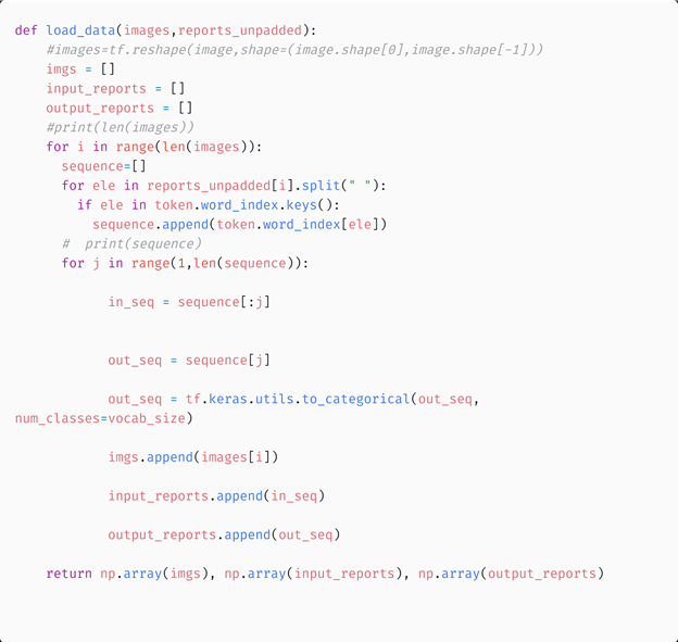
Training of the model
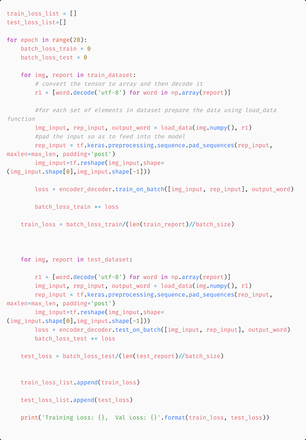
The data for training is prepared using the load data function.
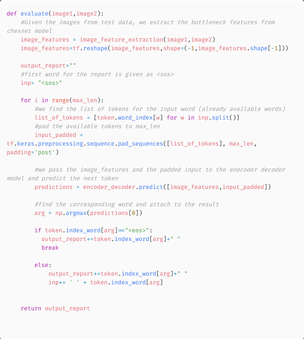
Evaluating the model using Greedy Search Algorithm
A greedy search algorithm builds up a solution piece by piece, always choosing the next piece that offers the most obvious and immediate benefit. Here the prediction is done through the following steps:
- For a given patient, get the image features using the encoder model
- Pass the encoder output and the token_index of the word “<sos>” (start of the sentence) to the decoder model and this will predict the probability distribution of each word across the vocabulary. We select the word with maximum probability as the next word
- The predicted word along with the input to the decoder is the next input sentence
- Step 2 and 3 are repeated till the word “<eos>” (end of the sentence) is reached.
Results from the model:
Example 1: ACTUAL REPORT: <sos> cardiac and mediastinal contours are within normal limits. the lungs are clear. bony structures are intact. <eos>
GENERATED REPORT: the heart normal size. the mediastinum unremarkable. the lungs are clear. <eos>
Example 2: ACTUAL REPORT: <sos> hyperinflated lungs with flattened diaphragm and increased retrosternal airspace. alveolar consolidation findings pleural effusion pulmonary edema. heart size within normal limits. right hilar calcification suggests previous granulomatous process. <eos>
GENERATED REPORT: the heart size and mediastinal silhouette are within normal limits for contour. the lungs are clear. pneumothorax pleural effusions. the are intact. <eos>
We can see that the model is performing poorly for longer sentences. The model fails to detect the medical condition.
We can use the BLEU score for evaluating the similarity between the generated and actual sentence. Let us analyze the performance of the model by calculating the overall bleu score for test data.
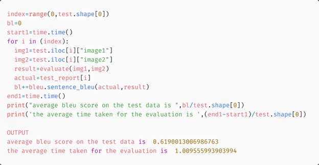
Now let us move on to a more advanced model.
Model 2: Encoder decoder model with attention
Attention Mechanism
The problem with the previous method is that, when the model is trying to generate the next word of the caption, this word is actually describing only a part of the image. But in the former approach, the generation of each word was based on the whole representation of the image. This is where the attention mechanism is useful. It helps to focus on some parts of the image while generating a particular word. Suppose the kth word in the actual output sequence is a description of some particular portion of the x-ray but not the whole x-ray image. So if we use the whole image for generating the kth word from the decoder, the required word might not be generated. Instead, if we use an attention mechanism to focus on some part of the image at a time, then results will improve.
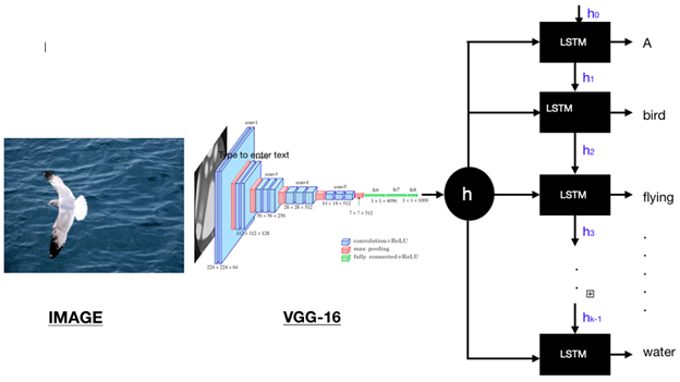
In the above figure, if we need to generate the word “bird” we need to focus on the pixels containing birds in the image. This is done using attention weights which gives a weightage to each part of the image. These weights are learned during training. You can learn more about the attention mechanism here.
Attention-based model
This model also has an encoder-decoder architecture. The encoder is the same as in the previous model, but the decoder has an extra attention unit in it.
Let us see how this attention-based model is working.
- Extract image features from CheXNet model
- Pass the features to the encoder model which gives the encoder output
- The encoder output and the previous decoder hidden state are passed to the attention model which calculate the attention weights
- The attention weights and encoder output are used to calculate the context vector
- The context vector and embedding vector of the previous decoder input are concatenated and passed to the GRU unit
- The GRU output is passed to the final dense layer
This is the flow through the model. The below figure will help to get a better understanding of this.
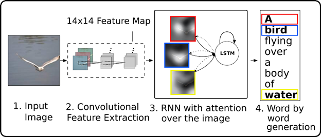
Figure 5: The architecture of attention-based encoder-decoder model for image captioning
Now let us try to understand each of these units
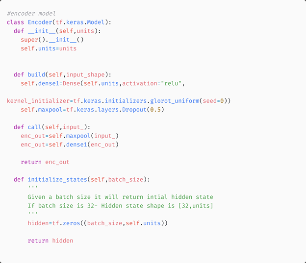
Encoder class
The encoder class will convert the image features from the CheXNet model into a lower-dimensional tensor
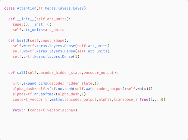
Attention Class
The attention class will use the previous hidden state of the decoder model and the encoder output to calculate the attention weights and context vector.
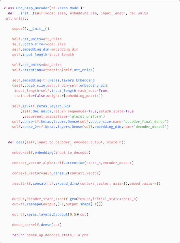
One step decoder and decoder classes
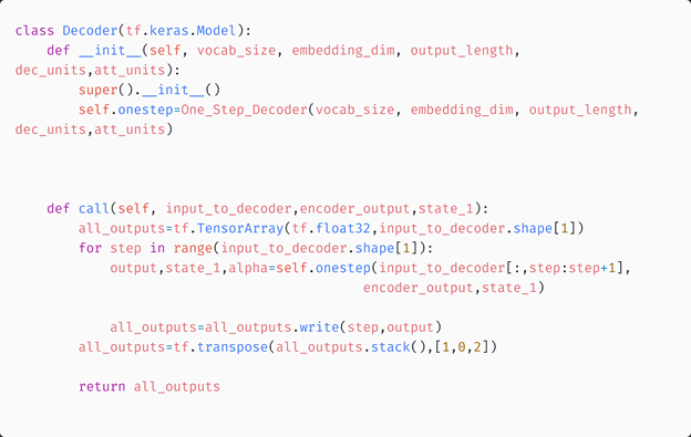
One step decoder class will perform the decoding of the encoder outputs. The decoder class will call this one step decoder at every time step. One step decoder, in turn, calls the attention model and returns the final output at that time step.
Each output word predicted by the one-step decoder is stored using the final decoder model and the final output sentence is returned.
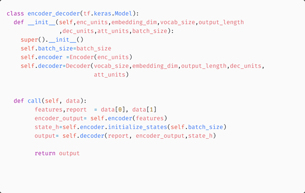
Encoder-Decoder Model
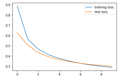
The below plot shows the train and test loss of the model
Results from Greedy search Algorithm
Example1:
ACTUAL REPORT: <sos> the lungs are clear. there pleural effusion pneumothorax. the heart and mediastinum are normal. the skeletal structures are normal. <eos>
GENERATED REPORT: the heart size and pulmonary vascularity appear within normal limits. the lungs are clear. there pleural effusion pneumothorax. <eos>
Example 2:
ACTUAL REPORT: <sos> the trachea midline. cardiomediastinal silhouette normal size and contour. the lungs are clear without evidence acute infiltrate effusion. there pneumothorax. the visualized bony structures reveal acute abnormalities. <eos>
GENERATED REPORT: the heart size and pulmonary vascularity appear within normal limits. the lungs are clear. there pleural effusion pneumothorax. <eos>
Here also, we can see that the model is not predicting well for longer sentences. The overall bleu score calculated for the test data using the greedy search algorithm is shown below

Evaluating the model using BeamSearch Algorithm
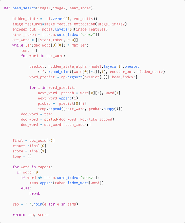
Let us predict the sentences using the Beam Search Algorithm. Instead of greedily choosing the most likely output for the next step, the beam search expands all possible outcomes and keeps the k most likely or probable outputs. Here k is known as the beam width, is a user-specified parameter, and it controls the number of beams or parallel searches through the sequence of probabilities. k=1 is nothing but a greedy search algorithm itself. As k increases the performance of the model can be improved, but the time complexity can be increased. So it is a choice between performance and time complexity.
In this case study, we consider k=3.
Example:
ACTUAL REPORT: heart normal size. the mediastinum unremarkable. the lungs are clear. evidence active tuberculosis. <eos>
GENERATED REPORT: <sos> heart size and lateral views the heart size and mediastinal contours are within normal pulmonary edema.
Here the reports have some common words, but they are still different. Also, the model is not able to predict tuberculosis which was present in the actual report. Now let us calculate the overall blue score of the test data.
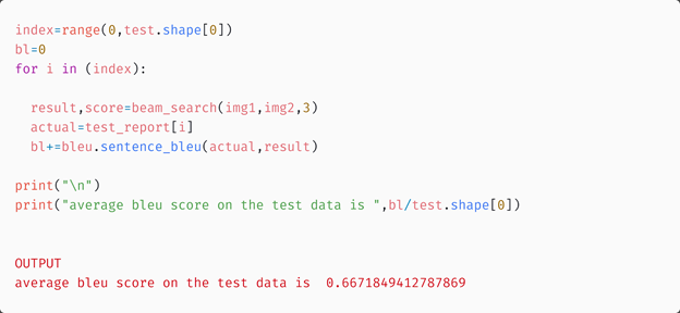
The results were improved when the beam search algorithm was used. But we expected the attention model to perform much better and here we are getting only a slight improvement in Bleu score. But why does this happen?
While extracting the image features from the Chexnet model, we used average pooling before the final layer which flattened the vector and ignored all the spatial features.

So the attention mechanism was done using the flattened vector. This might be the reason that we are not getting improved results. Now let us preserve the spatial information of the images and perform the attention mechanism.
Model 3: Using spatial image features on Model 2
Here we preserve the spatial information of the images while extracting the features from the CheXNet model. This allows the model to identify spatial patterns (edges, shading changes, shapes, objects, etc). Now let us understand the output from the CheXNet model.
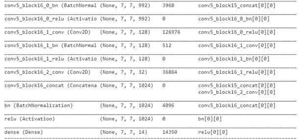
We can see that the final global average pooling layer is removed and the spatial information is retained. We remove the last activation layer to obtain the bottleneck features. So for every input image, we will get a (7,7,1024) dimensional vector as the output. Since we have two images per patient, we will concatenate these features to get a (7,14,1024) dimensional tensor as the final feature vector. Here 7 and 14 represent the actual locations that correspond to certain portions in the image, and 1024 indicate the depth. We can think of it as (7*14) locations each having a 1024 dimensional representation. So we reshape the tensors into (98,1024).
Model architecture and training of the model
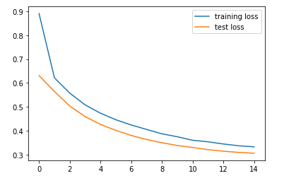
The model architecture and the training process is the same as the previous model, with the only difference in the dimension of input image features. The below graph shows the train and test losses of the model.
Evaluation using Beam search
Example 1:
ACTUAL REPORT: <sos> the lungs are clear. there pleural effusion pneumothorax. the heart and mediastinum are normal. the skeletal structures are normal. <eos>
GENERATED REPORT: <sos> heart size within normal limits. lungs are clear. there pleural effusion.
Example 2:
ACTUAL REPORT: <sos> heart and mediastinum within normal limits. negative for focal pulmonary consolidation pleural effusion pneumothorax. <eos>
GENERATED REPORT: <sos> heart size within normal limits. there pneumothorax pleural effusion pneumothorax.
In the first example, the generated report matches the original report. But in the second case, the generated report indicates the presence of pleural effusion but the actual report is showing negative for the same. Now let us calculate the overall blue score of the test data.

We can see that the results have improved when compared to the previous models. Also, The time for evaluation is more when the beam search is used. Now, let us modify this model slightly.
Model 4: Using bidirectional GRU on Model 3
In the previous model, we have used a unidirectional GRU in the decoder class. This yields good results, but what if we can improve this?
Let us consider Bidirectional GRU. Bidirectional GRUs have only input gate and forget gate. It allows for the use of information from both previous time steps and later time steps to make predictions about the current state. The model architecture and training are the same as that of the previous model with the only difference being that the decoder GRU is replaced by a Bidirectional one.
Let us look at the train and test losses of this model.
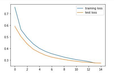
We can see that the losses are less when compared to the previous models.
Evaluation using Beam search
Example 1:
ACTUAL REPORT: <sos> heart size and vascularity normal. these contour normal. lungs clear. pleural effusions pneumothoraces. <eos>
GENERATED REPORT: <sos> the mediastinum within normal size and pleural effusion pneumothorax.
Example 2:
ACTUAL REPORT: <sos> the heart pulmonary and mediastinum are within normal limits. there pleural effusion pneumothorax. there focal air space opacity suggest pneumonia. there are minimal degenerative changes the spine. <eos>
GENERATED REPORT: <sos> the mediastinum within normal size and focal airspace disease.
The performance of the model has improved when compared to the previous models. In the first example, the generated report is almost the same as the actual report and the model is able to predict the medical condition of the person correctly. In the second example, the model predicted the medical condition partially. We can see that it is able to recall focal airspace disease or pneumonia, but is unable to predict pneumothorax. Still, the model performed better than the other models. Let us see the improvement in Bleu score.

9. Comparison of Models
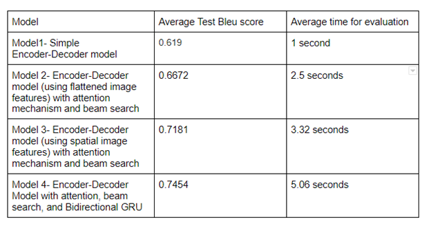
The below table shows a comparison between the models, based on the bleu score on test data and average evaluation time. We can see that the final model performed better than the others.
10. Model Deployment
You can see the demo video of the app here. The code for model deployment is available in my Github Repository.
11. Future Works
- We didn’t have a big dataset for this task. A larger dataset will produce better results
12. Profile
You can find my complete solution in my Github Repository and if you have any suggestions, please contact me via Linkedin
13. References
- https://www.appliedaicourse.com/course/11/Applied-Machine-learning-course
- https://towardsdatascience.com/image-captioning-in-deep-learning-9cd23fb4d8d2
- https://towardsdatascience.com/image-captioning-using-deep-learning-fe0d929cf337
- https://medium.com/analytics-vidhya/automatic-medical-report-generation-from-x-ray-images-through-ai-fd04de21e0e5
- https://machinelearningmastery.com/develop-a-deep-learning-caption-generation-model-in-python/
